
[This is an article, which is something I’ve optimized for readability and transmission of ideas, opposed to notes that are the seed of an idea and something I’ve written quickly.]
In Causality For Physics, I introduced Pearlian interventions for physical systems that evolve over time. In Physical Information, I defined what it means for a system to have information. Here, I will merge these threads and talk about what it means for a system to have causal effect, and the connection with information.
Review
$$
\newcommand{\0}{\mathrm{false}}
\newcommand{\1}{\mathrm{true}}
\newcommand{\mb}{\mathbb}
\newcommand{\mc}{\mathcal}
\newcommand{\mf}{\mathfrak}
\newcommand{\and}{\wedge}
\newcommand{\or}{\vee}
\newcommand{\es}{\emptyset}
\newcommand{\a}{\alpha}
\newcommand{\s}{\sigma}
\newcommand{\t}{\tau}
\newcommand{\T}{\Theta}
\newcommand{\D}{\Delta}
\newcommand{\o}{\omega}
\newcommand{\O}{\Omega}
\newcommand{\x}{\xi}
\newcommand{\z}{\zeta}
\newcommand{\fa}{\forall}
\newcommand{\ex}{\exists}
\newcommand{\X}{\mc{X}}
\newcommand{\Y}{\mc{Y}}
\newcommand{\Z}{\mc{Z}}
\newcommand{\P}{\Psi}
\newcommand{\y}{\psi}
\newcommand{\p}{\phi}
\newcommand{\l}{\lambda}
\newcommand{\B}{\mb{B}}
\newcommand{\m}{\times}
\newcommand{\N}{\mb{N}}
\newcommand{\R}{\mb{R}}
\newcommand{\I}{\mb{I}}
\newcommand{\H}{\mb{H}}
\newcommand{\e}{\varepsilon}
\newcommand{\Env}{\mf{E}}
\newcommand{\expt}[2]{\mb{E}_{#1}\left[#2\right]}
\newcommand{\set}[1]{\left\{#1\right\}}
\newcommand{\par}[1]{\left(#1\right)}
\newcommand{\vtup}[1]{\left\langle#1\right\rangle}
\newcommand{\Mid}{\,\middle|\,}
\newcommand{\abs}[1]{\left\lvert#1\right\rvert}
\newcommand{\inv}[1]{{#1}^{-1}}
\newcommand{\ceil}[1]{\left\lceil#1\right\rceil}
\newcommand{\dom}[1]{_{\mid #1}}
\newcommand{\df}{\overset{\mathrm{def}}{=}}
\newcommand{\M}{\mc{M}}
\newcommand{\up}[1]{^{(#1)}}
\newcommand{\Dt}{{\Delta t}}
\newcommand{\tr}{\rightarrowtail}
\newcommand{\tx}{\prec}
\newcommand{\qed}{\ \ \blacksquare}
\newcommand{\c}{\overline}
\newcommand{\A}{\mf{A}}
\newcommand{\cA}{\c{\mf{A}}}
\newcommand{\fB}{\mf{B}}
\newcommand{\cB}{\c{\mf{B}}}
\newcommand{\dg}{\dagger}
\newcommand{\Do}{{\mathrm{do}}}
\newcommand{\do}[2]{\underset{#1\leadsto #2}{\mathrm{do}}}
\newcommand{\lgfr}[2]{\lg\par{\frac{#1}{#2}}}
\newcommand{\sys}[2]{\left[#2\right]_{#1}}
\require{cancel}
$$
Information
This is a review of Bayesian information theory.
For possibility set $\O$ and subset $R\subseteq \O$, I define information as the narrowing-down of $\O$ to $R$, represented by the tuple
$$
\O \tr R \df (\O,R)\,.
$$
Suppose some $\o^*\in\O$ is the true possibility. Then the information $\O \tr R$ corresponds to the knowledge that $\o^* \in R$ and $\o^* \notin \O\setminus R$. Any set $A\subseteq\O$ is true iff $\o^*\in A$, and false otherwise.
Given a measure $\mu$ on $\O$ (need not be normalized), the information $\O\tr R$ is quantified by
$$
h(R) \df \lgfr{\mu(\O)}{\mu(R)}\,,
$$
which is the number of halvings to go from $\mu(\O)$ to $\mu(R)$.
Given the sets $R, D \subseteq \O$ where $D$ is to be regarded as a domain that we are narrowing down $\O$ to, the information $D \tr R\dom{D}$ is quantified by
$$
h(R \mid D) \df \lgfr{\mu(D)}{\mu(R\dom{D})}\,.
$$
where
$$
R\dom{D} \df R \cap D
$$
is a shorthand for set intersection, which makes clear that we are restricting set $R$ to domain $D$.
The information $\O\tr D$ is quantified by $h(D)$ which decomposes into
$$
h(D) = h(R \mid D) + i(R, D)\,,
$$
where the pointwise mutual information (PMI) is defined as
$$
i(R, D) = \lgfr{\mu(R\dom{D})\mu(\O)}{\mu(R)\mu(D)}\,.
$$
In other words, the information quantity $h(D)$ (due to the domain restriction $\O\tr D$), is the sum of information about $D$ and information missing about $D$.
If $i(R, A) = h(A)$, then $R \subseteq A$ and so the information $\O\tr R$ implies certainty that $A$ is true.
If $i(R, A) = 0$, then $R \subseteq A$ contains no information about whether $A$ is true.
If $i(R, A) < 0$, then information is lost about whether $A$ is true due to the information $\O\tr R$, i.e. $\O\tr R$ contains information about whether $A$ is false.
If $i(R, A) = -\infty$, then $R \cap A = \es$ and $\O\tr R$ implies certainty that $A$ is false, i.e. an infinite amount of information would be needed to have certainty that $A$ is true.
See Information Algebra for further intuition on the meaning of PMI.
I use $h(A \tr B) \df h(B \mid A)$ as a shorthand for quantity of the information $A \tr B$. Note that $h(\O \tr B) = h(B \mid \O) = h(B)$.
Physical Systems
Continuing from Physical Information, let $\t_\Dt$ for $t\in\R$ be a family of bijective time-evolution functions on the universe’s state space $\O$ which form the group $(\set{\t_\Dt \mid \Dt\in\R}, \circ)$, where “$\circ$” is the function composition operator. Any system is defined by its state space, which is a partition on $\O$. For example, system A has state space $\mf{A}$, where each element $a\in\mf{A}$ is a possible state of the system, and $a\subseteq\O$ is the set of all states of the universe for which system A is in the same state $a$. State equivalence w.r.t. system A induces an equivalence relation on $\O$ where $\mf{A}$ is the set of equivalence classes:
$$
\sys{\mf{A}}{\o} = a\,\,\mathrm{s.t.}\,\,\o\in a
$$
A partition complement of $\A$, denoted $\cA$ (if one exists), satisfies the following properties:
- $\cA$ is a partition of $\O$.
- $\I(\A, \cA) = 0$,
- $\A\otimes\cA = \mf{O} = \set{\set{\o}\mid\o\in\O}$,
where $\A\otimes\cA = \set{a\cap a^\dg \mid a\in\A \and a^\dg\in\cA}$ is the partition product of $\A$ and $\cA$, and $\mf{O}$ is the singleton partition of $\O$, which can be thought of as the universe’s state space. $\cA$ is the state space of system A’s environment, which is everything in the universe outside of system A.
Interventions
In Causality For Physics, I introduced the intervention on a trajectory of a system. Let $\s:\R\to\O$ be a trajectory, which is a function from time to states s.t. $\s(t+\Dt) = \t_\Dt(\s(t))$ for all $t,\Dt\in\R$. We say that $\s$ is $\t$-valid. An intervention at time $T$ is a surgery on $\s$, i.e. a modification to $\s$, s.t. $\s$ on the domains $(-\infty,T)$ and $(T,\infty)$ are each $\t$-valid, but $\s$ on the domain $(T-\e,T+\e)$ for $\e>0$ is not $\t$-valid.
The “do”-operator performs an intervention on trajectory $\s$ given state-replacement function $I : \O\to\O$,
$$
\do{I}{T}[\s](t) \df \begin{cases}\s(t) & t < T \\ \t_{t-T}(I(\s(T))) & t\geq T\end{cases}\,.
$$
Let $I_\o = \_\mapsto \o$ be the constant state-replacement function that outputs $\o$, and define $\s_\o$ to be the trajectory s.t. $\s_\o(T) = \o$. Then
$$
\do{I_\o}{T}[\s](t) = \begin{cases}\s(t) & t < T \\ \s_\o(t) & t\geq T\end{cases}\,.
$$
Intervention Sets
Judea Pearl defines causal effect as the set of all changes resulting from all possible interventions on a variable (see Causality For Physics for details). To characterize causal effect in physical systems, it follows that we should consider a set of interventions taken at some time $T$ in parallel (so to speak). Specifically, an intervention set is a set of states, $J\subseteq\O$, representing the set of simultaneous interventions that set the universe’s state at time $T$ to every $\o\in J$,
$$
\mc{J}_\Do = \left\{\do{I_\o}{T} \,\middle|\, \o\in J\right\}\,.
$$
This set of interventions applied to a trajectory $\s$ results in the set of modified trajectories,
$$
\mc{J}_\Do\s = \left\{\par{t\mapsto\begin{cases}\s(t) & t < T \\ \s_\o(t) & t\geq T\end{cases}} \,\middle|\, \o\in J\right\}\,.
$$
The set of states $E_\Dt = \left[\mc{J}_\Do\s\right](T+\Dt)$ for $\Dt > 0$ is called the effect set of the intervention set $J$ at time $T+\Dt$. Notice that $E_\Dt = \t_\Dt(J)$.
Because time-evolution is Markovian (state at time $t$ only depends on state at $t-\e$ for arbitrarily small $\e>0$), we can entirely disregard the pre-intervention trajectory $\s$. The effect set $E_\Dt$ (for every $\Dt > 0$) fully characterizes the effect $\Dt$ into the future of the intervention set $J$. Because $E_\Dt$ depends only on $J$ and not the trajectory $\s$, we can bypass the “do”-operator entirely and just work with intervention sets and effect sets.
With this simplification, we can just as easily perform retro-causal interventions. That is to say, $E_\Dt = \t_\Dt(J)$ where $\Dt < 0$ is also an effect set, i.e. the set of retro-effects due to intervening at time $T$ and propagating the changes into the past. Furthermore, $E_0 = \t_0(J) = J$ is also an effect set, and I consider an intervention to be its own simultaneous effect at the time the intervention is taken.
Interventions that propagate causal effects into the past and future are bidirectional. In the case of trajectories, a bidirectional intervention that sets time $T$ to state $\o$ replaces $\s$ with the alternative trajectory $\s_\o$, completely erasing any trace of $\s$. Bidirectional interventions don’t perform surgeries, losing the key feature of Pearlian interventions. If you are suspecting that this kind of intervention is merely conditionalization, you are correct. Because our time-evolution is Markovian and we are conditioning on a node in the Markov chain (the Markov blanket), the “do”-operator and conditionalization are equivalent operations (see Causality For Physics).
From here on, I’ll only work with intervention sets and effect sets, leaving out mention of the “do”-operator and surgeries on trajectories entirely.
Quantifying Causal Effect
Interventions on causal models are usually taken from the 1st person perspective, i.e. the perspective of a human or “agent” that is trying to decide what to do in the world. I’ll start from that perspective, and then shift to a 3rd person perspective where interventions are w.r.t. systems within the model.
Suppose we (the creators of this physical model) know that the universe is in state $\o\up{t}$ at time $t$. Then we have the information $\O\tr\set{\o\up{t}}$ about time $t$, and the information $\O\tr\set{\t_\Dt(\o\up{t})}$ about time $t+\Dt$.
Applying the intervention set $J$ at time $t$ means that now the universe can be in any of the states in $J$ (or all of them at the same time if you prefer to think of it that way). Our information about the state of the universe at time $t$ has been reduced to $\O\tr J$, and $\O\tr \t_\Dt(J)$ about the state at time $t+\Dt$.
Regarding information quantities, we started with $h\par{\set{\o\up{t}}}$ bits (certainty that the universe is in state $\o\up{t}$), and the intervention set $J$ reduced our information to $h(J)$ bits, for an information loss of $h\par{\set{\o\up{t}}} - h(J) = \lgfr{\mu(J)}{\mu\set{\o\up{t}}}$ bits. This is the number of doublings it takes to expand the set $\set{\o\up{t}}$ out to $J$, just as $h(J)$ is the number of halvings it takes to narrow down $\O$ to $J$.
In general, let $E = \t_\Dt(J)$ be an effect set. $E$ replaces $\o\up{t+\Dt}$ as the state of the universe at time $t+\Dt$, which we can view as expanding out the singleton set $\set{\o\up{t+\Dt}}$ to $E$, which requires $\lgfr{\mu(E)}{\mu\set{\o\up{t+\Dt}}}$ doublings, and is also the quantity of information lost about what state the universe is in at time $t+\Dt$. I call this the quantity of causal effect of $E$.
Note that we can write this quantity more succinctly as $\lg\nu_{\o\up{t+\Dt}}(E)$, which now looks like the log-size of $E$, where the measure $\nu_\o(E) = \mu(E)/\mu\set{\o}$ is defined as a rescaling of $\mu$ so that $\o$ has the unit size. In this sense, $\o$ serves as a reference for choice of units when computing the size of $E$. If $\mu$ is uniform (i.e. $\mu\set{\o} = \mu\set{\o'}$ for all $\o,\o'\in\O$), then $\o$ is irrelevant for calculating the log-size, and we have $\lg\nu(E) = \lg\mu(E) - u$ where $u=\lg\mu\set{\o}$ is a constant. Furthermore, if $\mu$ is the counting measure, then $\lg\nu(E) = \lg\abs{E}$.
Information Algebra Review
In Information Algebra, I gave the intuition that pointwise mutual information (PMI), $i(A, D)$, quantifies the amount by which the information needed to have certainty about $A$ is reduced by having $\O\tr D$. PMI is also the negative change in information due to replacing $\O\tr A$ with $D \tr A\dom{D}$:
$$
\begin{aligned}
i(A, D) &= -(h(D \tr A\dom{D}) - h(\O\tr A)) \\
&= h(A) - h(A \mid D)\,.
\end{aligned}
$$
The conditional information, $h(A \mid D)$, quantifies the remaining amount of information needed to have certainty about $A$, given $\O\tr A$. Conditional information is the change in information due to replacing $\O\tr D$ with $\O\tr A\dom{D}$:
$$
\begin{aligned}
h(A \mid D) &= h(\O\tr A\dom{D}) - h(\O\tr D) \\
&= h(A\cap D) - h(D)\,.
\end{aligned}
$$
Their sum of $i(A,D)$, the information had about whether $A$ is true, plus $h(A\mid D)$, the information still needed to know that $A$ is true, is the total quantity of information $h(A)$ about whether $A$ is true:
$$
h(A) = i(A, D) + h(A\mid D)\,.
$$
Effect Algebra
Above I defined the quantity of causal effect due to effect set $E$ as $\lg\mu(E) - u$ where $u$ is some normalization constant (which sets the unit size for the scaled measure $\nu$). I used singleton sets of the form $\set{\o}$ as references for the unit size, i.e. $u = \lg\mu\set{\o}$.
In general, any set $A\subseteq\O$ can be a reference for scaling $\mu$. The quantity of the causal effect $E$ relative to $A$ is
$$
\begin{aligned}
\lg\mu(E) - \lg\mu(A) &= \lg\par{\frac{\mu(E)}{\mu(A)}\cdot\frac{\mu(\O)}{\mu(\O)}}\\
&= h(A) - h(E) \\
&= -(h(\O\tr E) - h(\O\tr A))\,.
\end{aligned}
$$
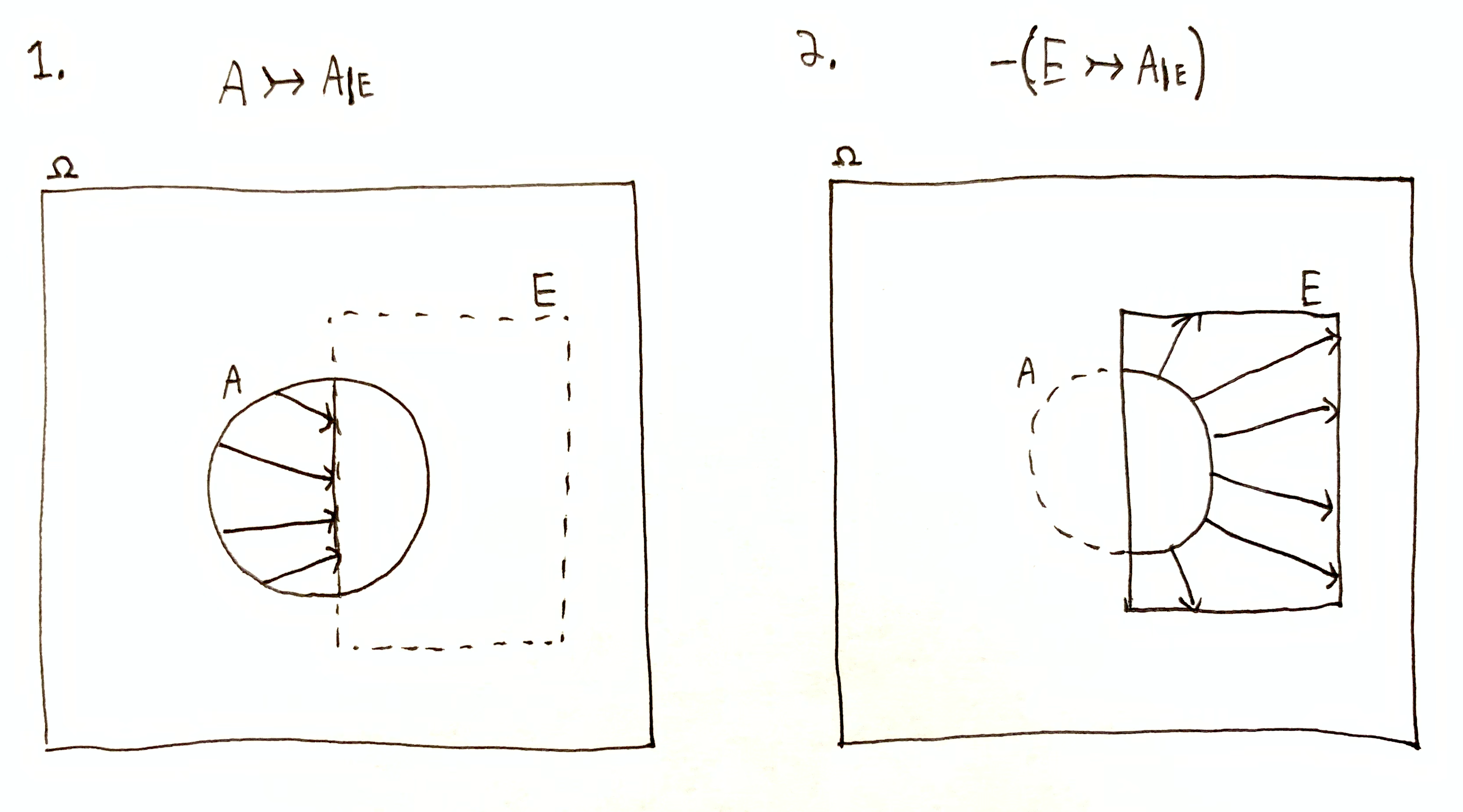
This is simply the change in information quantity due to replacing $\O\tr A$ with $\O\tr E$, i.e. the net information change due to replacing $A$ with $E$. This replacement operation can be decomposed into two steps:
- Narrowing down $A$ to $A\dom{E}$, for an information gain of $h(A \tr A\dom{E}) = h(A\dom{E} \mid A) = h(E \mid A)$ halvings.
- Expanding out $A\dom{E}$ to $E$, for an information loss of $h(E \tr A\dom{E}) = h(A \mid E)$ doublings.
Quantity of causal effect is their difference:
$$
\begin{aligned}
h(A) - h(E) &= \cancel{i(A, E)} + h(A \mid E) - (\cancel{i(E, A)} + h(E \mid A))\\
&= h(A \mid E) - h(E \mid A) \\
&= h(E \tr A\dom{E}) - h(A \tr A\dom{E})\,.
\end{aligned}
$$
So for any $A$, the total quantity of effect relative to $A$ (rescaling scaling so that $\nu(A) = 1$) equals the information lost about $A$ due to effect $E$ minus the information gained about $A$ due to effect $E$.
If $A \subseteq E$, then $h(A) - h(E) = h(A \mid E)$.
Combined replacement operation, going from $A$ to $E$. Two step replacement operation: 1. Narrowing down $A$ to $A\dom{E}$; 2. Expanding out $A\dom{E}$ to $E$.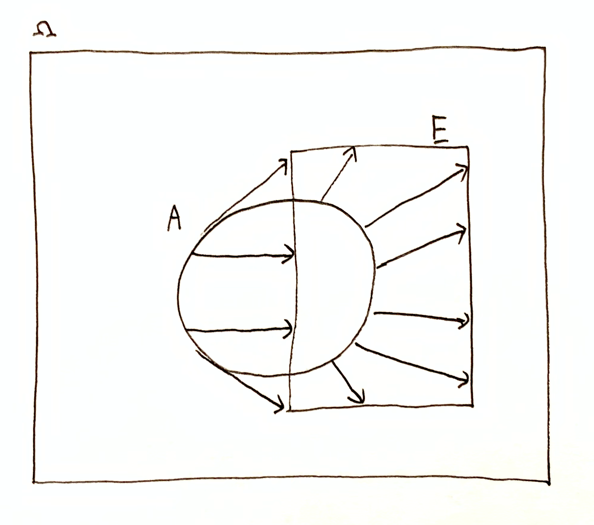
Effect-On
Just as $i(A,E)$ is the quantity of “information-about”,
$h(A \mid E)$ is quantity of “effect-on”.
$i(A,E)$ is the relative change in quantity of information needed to know that $A$ is true, due to gaining the information $\O\tr E$.
$h(A\mid E)$ is the quantity of information lost about whether $A$ is true due to the loss of information $E \tr \set{\o^*}$, where $\o^*$ is the true state (assuming $\o^* \in E$).
When I discuss intervention sets w.r.t. systems below, those intervention sets will always contain the true state of the universe.
Systems
Let $\o\up{t}\in\O$ be the true state of the universe at time $t$.
System A has state space $\A$ and system A’s environment has state space $\cA$, which is a partition complement of $\A$.
Let $a\up{t}=\sys{\A}{\o\up{t}}\in\A$ and $\c{a}\up{t}=\sys{\cA}{\o\up{t}}\in\cA$ be the states of system A and the environment respectively at time $t$.
Then $a\up{t}\cap\c{a}\up{t} = \set{\o\up{t}}$.
In the usual formulation of causality, an intervention is an action taken on the world by an agent. In my formulation, an intervention set $J$ is a collection of counterfactual states, i.e. states that the universe could be in. The effect of an intervention set is uncertainty about which state the universe is in, either in the past, present, or future. That is to say, causal effect is lack of information.
System A lacks information about the environment’s state, and so from system A’s perspective, the universe could be in any one of the states $\o \in a\up{t}$. This is logically equivalent to applying the intervention set $J = a\up{t}$ at time $t$. The effect $E = \t_\Dt(a\up{t})$ at time $t+\Dt$ is system A’s lack of information about time $t+\Dt$. Likewise, from the environment’s perspective, the universe can be in any of the states $\o\in\c{a}\up{t}$, and so on.
System A has the information quantity $h(a\up{t})$ at time $t$, but also the uncertainty quantity (lack of information) $h\par{\set{\o\up{t}} \Mid a\up{t}}$. They add up to the total information there is to have about the true state of the universe:
$$h\par{a\up{t}} + h\par{\set{\o\up{t}} \Mid a\up{t}} = h\par{\set{\o\up{t}}}\,.$$
If we consider the intervention set $J = a\up{t}$, then $h\par{\set{\o\up{t+\Dt}} \Mid \t_\Dt(a\up{t})}$ is the quantity of causal effect at time $t+\Dt$ due to replacing $\set{\o\up{t+\Dt}}$ with $\t_\Dt(a\up{t})$. By to conservation of information quantity, this quantity of causal effect is constant for all $\Dt\in\R$. This quantity is the total causal power of the environment from system A’s perspective. Likewise, $h\par{\set{\o\up{t}} \Mid \c{a}\up{t}} = h\par{\set{\o\up{t+\Dt}} \Mid \t_\Dt(\c{a}\up{t})}$ is the total causal power of system A, from the environment’s perspective.
Causal power is a constant through time, but can vary depending on which state $\o\in\O$ is true. That is to say, $h\par{\set{\o} \Mid \sys{\A}{\o}}$ need not equal $h\par{\set{\o'} \Mid \sys{\A}{\o'}}$ for $\o,\o'\in\O$, and likewise for $h\par{\set{\o} \Mid \sys{\cA}{\o}}$ and $h\par{\set{\o'} \Mid \sys{\cA}{\o'}}$.
Effect vs Information
In addition to system A and it’s environment, consider any system B with state space $\fB$.
Following from Physical Information, at time $t$, system A has the information quantity $i(b,\t_\Dt(a\up{t}))$ about whether some state $b\in\fB$ is true (contains $\o\up{t+\Dt}$) at time $t+\Dt$.
Also, from system A’s perspective at time $t$, the environment has the effect quantity $h(b \mid \t_\Dt(a\up{t}))$ on $b$ at time $t+\Dt$, which is the quantity of information system A is missing about whether $b$ is true (the quantity of information needed to have certainty that $b$ is true).
The total quantity of information there is to have about whether $b$ is true decomposes into information had about $b$ and information missing about $b$ (effect on $b$):
$$
h(b) = i(b, \t_\Dt(a\up{t})) + h(b \mid \t_\Dt(a\up{t}))\,.
$$
Likewise, system A’s environment (at time $t$) has the information $i(b,\t_\Dt(\c{a}\up{t}))$ about whether $b$ is true at time $t+\Dt$, and from its perspective, system A has the effect quantity $h(b \mid \t_\Dt(\c{a}\up{t}))$ on $b$ at time $t+\Dt$. We have the decomposition $h(b) = i(b, \t_\Dt(\c{a}\up{t})) + h(b \mid \t_\Dt(\c{a}\up{t}))$.
Note that if $b \cap \t_\Dt(a\up{t}) = \es$, then $i(b, \t_\Dt(a\up{t})) = -\infty$ and $h(b \mid \t_\Dt(a\up{t})) = \infty$, meaning that system A is missing an infinite quantity of information about whether $b$ is true, i.e. system A has certainty that $b$ is false. The effect of the environment on $b$ is infinite, meaning that the effect of varying the environment is to always make $b$ false. On the other hand, if $h(b \mid \t_\Dt(a\up{t})) = 0$, then $i(b, \t_\Dt(a\up{t})) = h(b)$ and the effect of varying the environment is to always make $b$ true, and thus system A has certainty that $b$ is true.
Sum-Conservation Laws
Analogous to Physical Information, quantity of causal effect decomposes into a conserved sum.
Let $E$ be an effect set and $b\in\fB$ be a possible state of system B such that $b \cap E$ is non-empty contains the true state $\o\in\O$. Then $h(\set{\o}) - h(E) = h(\set{\o} \mid E)$ is the total quantity of effect $E$, and $h(b \mid E)$ is the effect $E$ on $b$.
Suppose $h(b \mid E) < h(\set{\o} \mid E)$. Then we might ask, “where did the remaining effect go?”
Shrinking $b$ down to $b\cap c$ s.t. $b\cap c \subseteq E$, then we have $h(b\cap c \mid E) = \lg\mu(E) - \lg\mu(b\cap c)$, which is the quantity of causal effect $E$ using $b\cap c$ as the reference unit size. Furthermore, if $c$ is chosen so that $b\cap c = \set{\o}$, then $h(b\cap c \mid E) = h(\set{\o} \mid E)$ is the total quantity of effect $E$.
We have the following decomposition:
$$
\begin{aligned}
h(b\cap c \mid E) &= h(b \mid E) + h(b \mid c \cap E)\\
&= h(b \mid E) + h(c \mid E) - i(b, c \mid E)\,.
\end{aligned}
$$
Since $h(\cdot \mid \cdot)$ is always positive, $h(b\cap c \mid E) = h(b \mid E) + h(b \mid c \cap E)$ is a decomposition into positive terms. The next line, $h(b\cap c\mid E) = h(b \mid E) + h(c \mid E) - i(b, c \mid E)$ is a decomposition into the separate effects of $E$ on $b$ and $c$ individually, minus their interaction.
This nicely complements the information sum-law from Physical Information:
$$
i(b \cap c, E) = i(b, E) + i(c, E) - i(b, c, E)\,,
$$
where $i(b \cap c, E) = h(E)$ when $b \cap c \subseteq E$.
When added together, they form the combined decomposition:
$$
\begin{aligned}
h(b \cap c) &= i(b \cap c, E) + h(b\cap c \mid E) \\
&= (i(b, E) + i(c, E) - i(b, c, E)) + (h(b \mid E) + h(c\mid E) - i(b, c \mid E))\\
&= (i(b, E) + h(b \mid E)) + (i(c, E) + h(c \mid E)) - i(b,c) \\
&= h(b) + h(c) - i(b,c)\,.
\end{aligned}
$$
Self-Interventions
Going back to system A and its environment, with respective state spaces $\A$ and the partition-complement $\cA$, recall that $a^\dg \in \cA$ is both a state of system A’s environment and an intervention set varying system A while keeping the environment held fixed. From the environment’s perspective, system A has the effect set $E = \t_\Dt({a^\dg}\up{t})$, and the quantity of effect $h(a^\dg \mid E)$ on the environment state $a^\dg$, and $h(a \mid E)$ on system A’s state $a$.
We could ask, does system A have causal effect from system A’s perspective? At first this may seem like a contradiction of terms, since I defined the information that system A has to be exactly it’s current state. Causal effect of system A is due to lack of information about system A’s state.
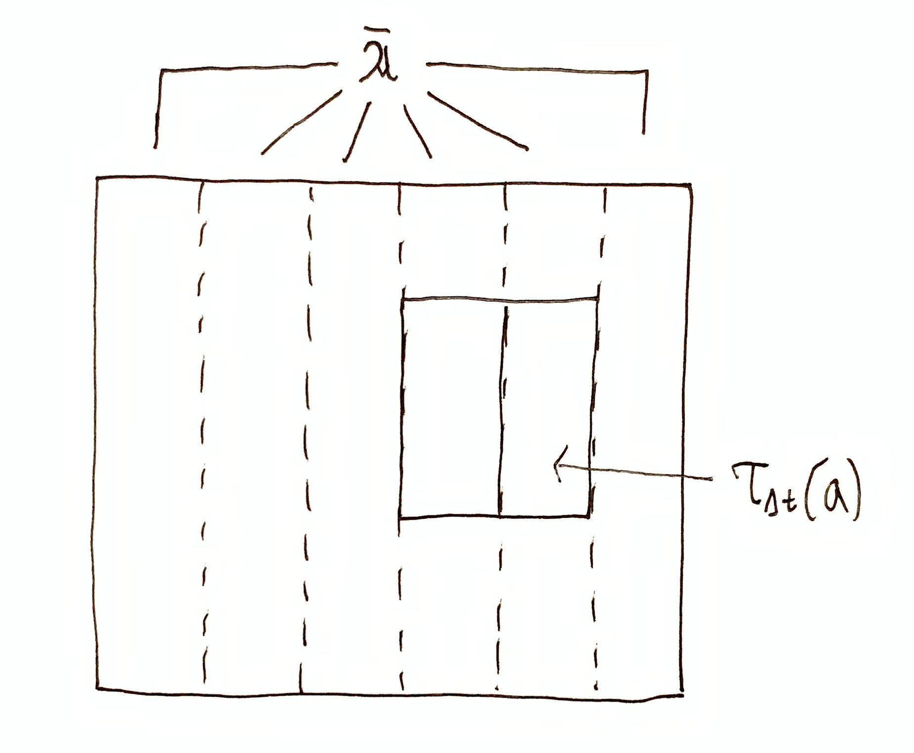
Just as in Physical Information I considered the narrowing down of a partition to a sub-partition, let’s now consider interventions on partitions rather than states. Specifically, replacing the single system-A state $a\up{t}$ (a subset of universe states $\O$) with the state set $\A$ (a partition of $\O$). Then $\A$ varies the state of system A, while also keeping the state of the environment unknown.
Let $\t_\Dt(\A) = \set{\t_\Dt(a) \mid a\in\A}$ be the time-evolved partition, i.e. the set of all of system A’s states time-evolved $\Dt$ into the future. Let’s motivate a measure of system A’s causal effect on the environment due to this new kind of intervention on partitions. Consider the following cases:
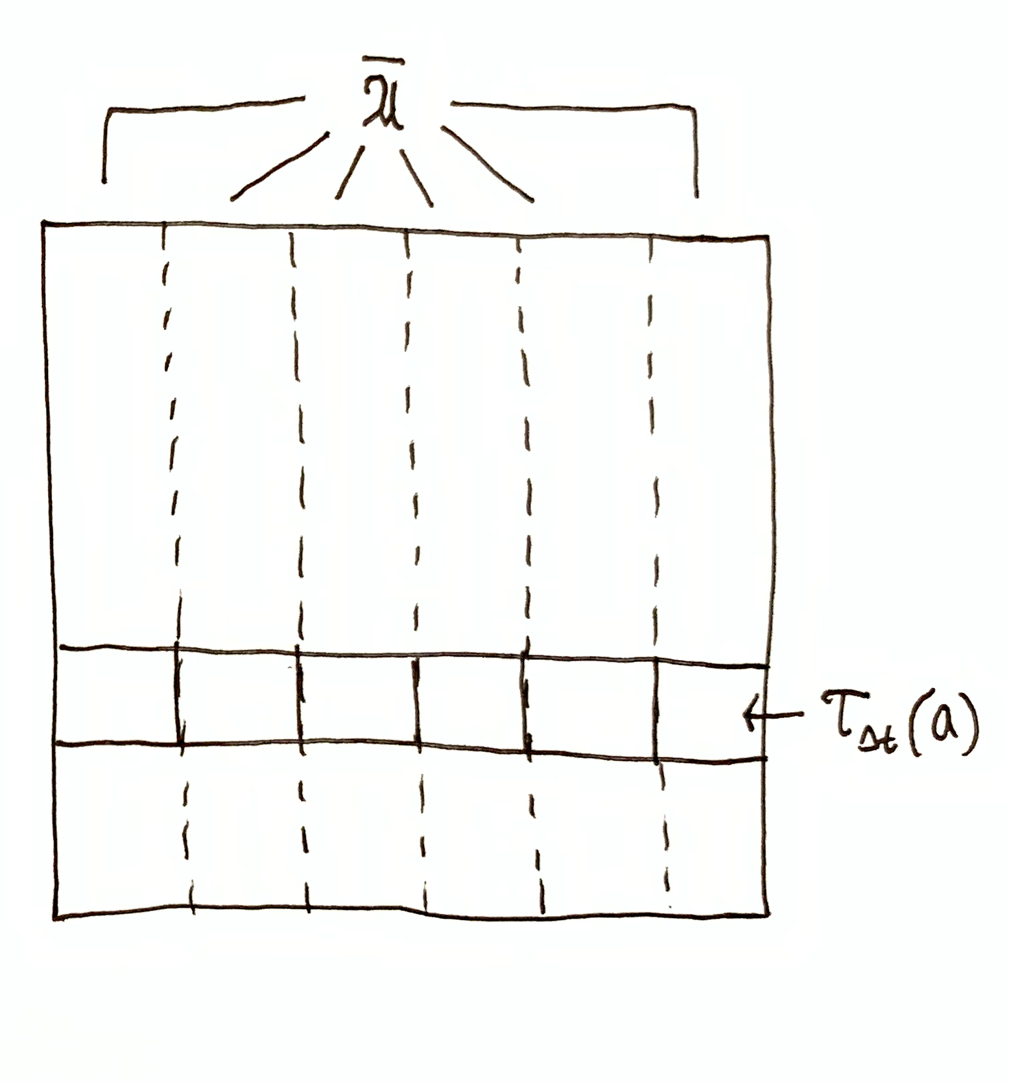
- $\t_\Dt(\A) = \cA$. Clearly system A’s state at time $t$ fully determines the environment’s state at time $t+\Dt$, and so system A’s effect on the environment is maximal.
- $\I(\cA, \t_\Dt(\A)) = 0$, i.e. $\cA$ and $\t_\Dt(\A)$ are orthogonal. Clearly system A’s state at time $t$ has no determination on the environment’s state at time $t+\Dt$, and system A has no effect on the environment.
- For some $a\in\A$, if the sub-partition $\cA\dom{\t_\Dt(a)} = \set{a^\dg\cap \t_\Dt(a) \Mid a^\dg\in\cA}$ contains multiple non-empty members, then that variation in the enviornment’s state given a particular state of system A is system A’s lack of determination of the environment’s state. That “lack of determination”, i.e. variation, can be quantified using $\H(\cA \mid \t_\Dt(a))$.
The case where $\t_\Dt(\A) = \cA$. The case where $\I(\cA, \t_\Dt(\A)) = 0$. The case where $\H(\cA \mid \t_\Dt(a)) > 0$, meaning there is some variation to the environment when system A’s state $a$ is held fixed. This is the part of the environment’s total variation $\H(\cA)$ that is not caused by system A.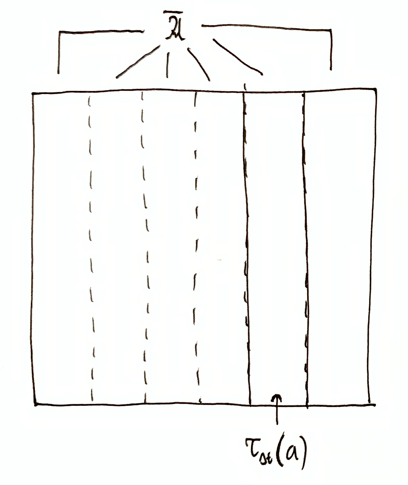
It should be becoming clear that
$$\I(\cA, \t_\Dt(\A))$$
is quantifying the summary effect of varying system A’s state on the environment, and $\H(\cA \mid \t_\Dt(\A))$ the remaining variation in the environment not due to system A, giving the total
$$
\H(\cA) = \I(\cA, \t_\Dt(\A)) + \H(\cA \mid \t_\Dt(\A))\,.
$$
This should be surprising, since I previously defined $i(a^\dg, \t_\Dt(a))$ as the information system A has (being in state $a$) about the environment state $a^\dg$ in the future, and $h(a^\dg \mid \t_\Dt(a))$ the effect of varying the environment on the environment’s state. Now, I’m saying that the expected PMI, $\I(\cA, \t_\Dt(\A))$, is quantifying the causal effect of system A on the environment.
This connection can be rigorously arrived at.
Let $R = \t_\Dt(a)$ and $R^\dg = \t_\Dt(a^\dg)$, and $b\subseteq\O$ is some set.
Note that if $a$ and $a^\dg$ are orthogonal and their intersection $a\cap a^\dg = \set{\o}$ is singleton, then the same is true for the time-evolved sets $R$ and $R^\dg$.
By plugging in $h(b) = i(b, R^\dg) + h(b \mid R^\dg)$ to $h(b) = i(b, R \cap R^\dg) = i(b, R) + i(b, R^\dg) + i(R, R^\dg\mid b)$, we get
$$
h(b \mid R^\dg) = i(b, R) + i(R, R^\dg\mid b)\,.
$$
Taking the expectation of both sides and replacing $b$ with the state of the environment, we get
$$
\H(\cA \mid \t_\Dt(\cA)) = \I(\cA, \t_\Dt(\A)) + \I(\t_\Dt(\A), \t_\Dt(\cA)\mid \cA)
$$
and all the terms are now guaranteed to be positive. Then we have the inequality,
$$
\H(\cA \mid \t_\Dt(\cA)) \geq \I(\cA, \t_\Dt(\A))\,,
$$
with equality when $\I(\t_\Dt(\A), \t_\Dt(\cA)\mid \cA) = 0$.
We can interpret $\H(\cA \mid \t_\Dt(\cA))$ as the average of $h(a^\dg \mid \t_\Dt(a'^\dg))$ across all $a^\dg, a'^\dg \in \cA$, which is the effect on env. state $a^\dg$ due to varying system A, while keeping the initial env. state fixed at $a'^\dg$. So the average effect of system A on the env., in this sense, is lower bounded by the summary effect, $\I(\cA, \t_\Dt(\A))$, of system A on the environment due to taking the partition $\A$ to be an intervention set (which does not specify that the environment is in any particular state).
The Information-Effect Cube
As before, system A has the state space $\A$ and its environment the partition complement $\cA$. Let $a\in\A$ be any system-A state, and $a^\dg\in\cA$ be any environment state. Let $R = \t_\Dt(a')$ and $R^\dg = \t_\Dt(a'^\dg)$ be the time-evolved states of system A and its environment.
$R$ can be regarded as either the information that system A has, $\O\tr R$, or the effect set due to varying the environment (intervention set $a$). Likewise, $R^\dg$ can be regarded as either the information that the environment has, $\O\tr R^\dg$, or the effect set due to varying system A (intervention set $a^\dg$).
So $i(a, R)$ is the information system A has about its own future state $a$, and $i(a, R^\dg)$ is the information the environment has about system A’s future state $a$. Likewise, $h(a \mid R)$ is the effect of the environment on system A’s future state $a$, and $h(a \mid R^\dg)$ is the effect of system A on system A’s future state $a$.
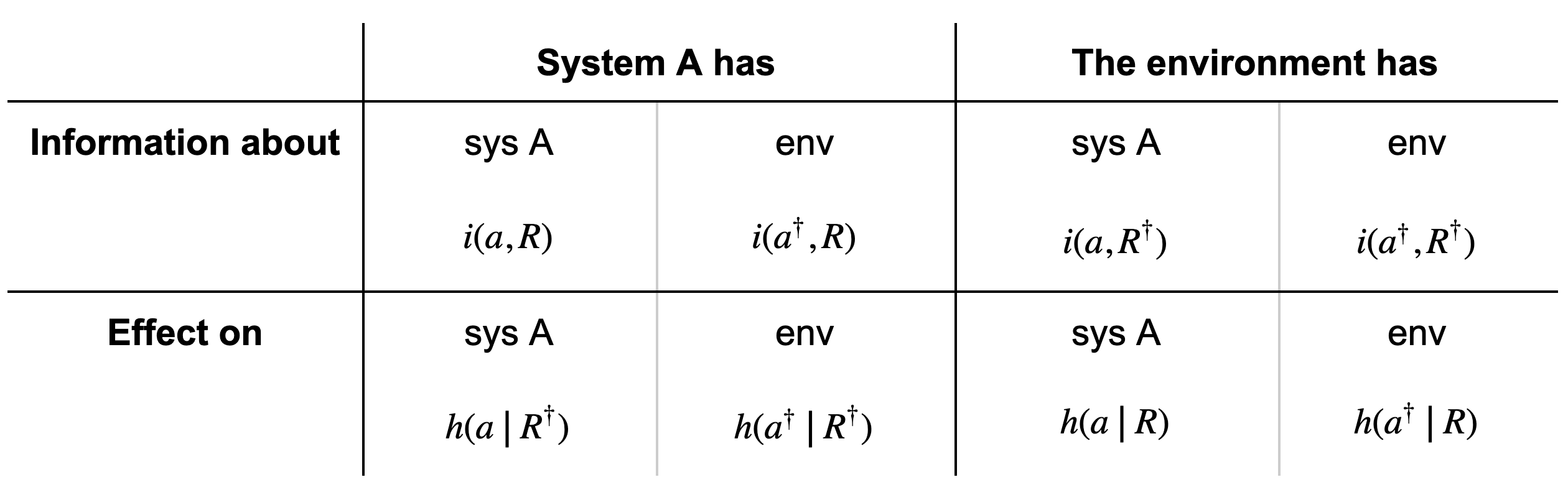
The table of all the possible permutations of $i \leftrightarrow h$, $a\leftrightarrow a^\dg$ and $R\leftrightarrow R^\dg$.
All of these quantities can be visualized together as the corners of a cube:
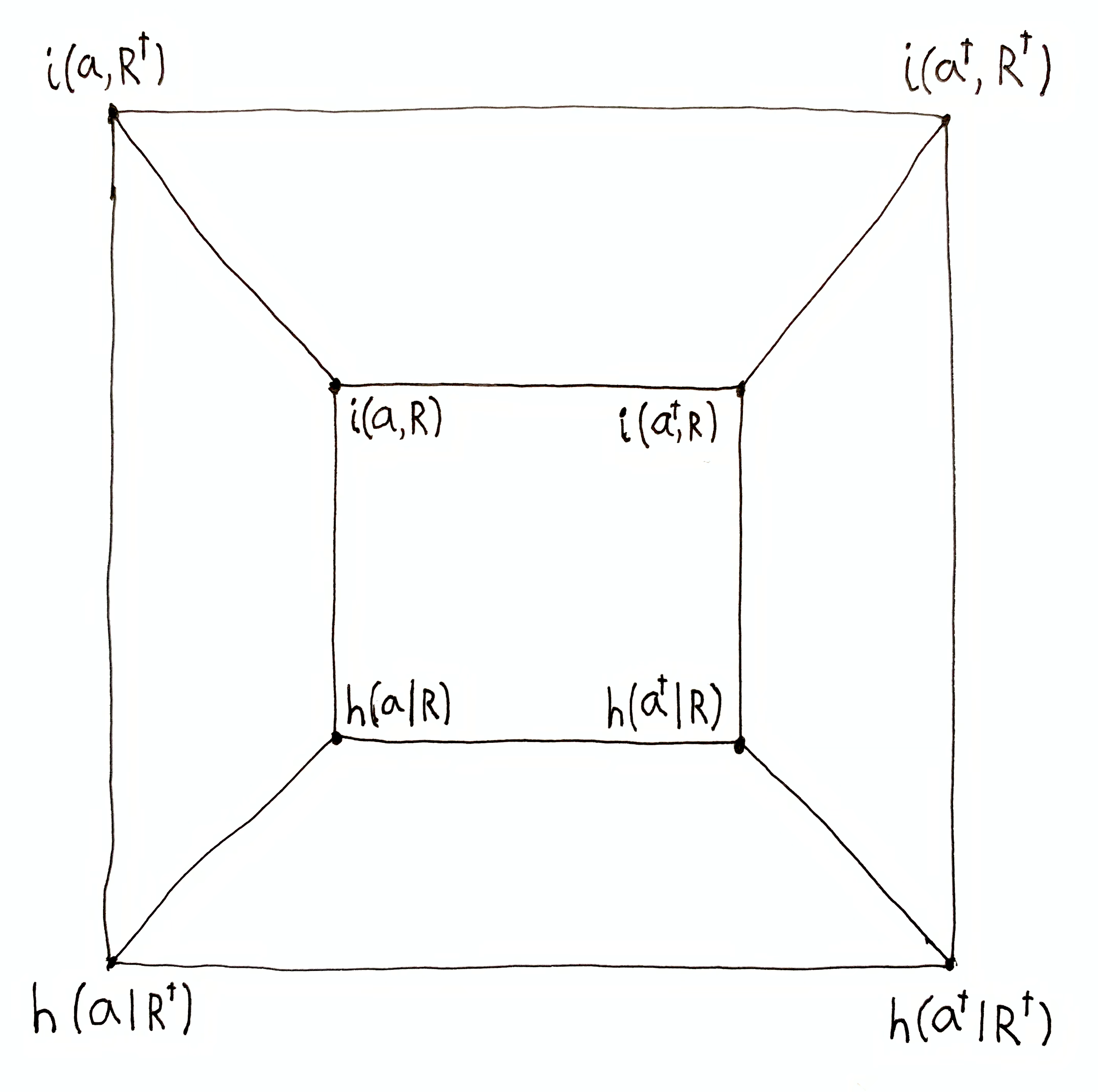
Ever pair of vertices has a corresponding identity linking the two, which can be useful for answering a number of questions about causality and information.
For example, the more information sys. A has about the env.’s future, the less information sys. A has about its own future? We can verify this using the identity $i(a^\dg, R) = h(R) - i(a, R) - i(a, a^\dg \mid R)$, assuming that $a\cap a^\dg \in R$. If all the other terms are held constant, then $i(a^\dg, R)$ and $i(a, R)$ are inversely related.
Here are a few more relationships:
- $i(a, R) = h(a) - i(a, R^\dg) - i(R, R^\dg \mid a)$, assuming $R \cap R^\dg \subseteq a$.
- $h(a \mid R) = i(a^\dg, R) + i(a, a^\dg\mid R)$
- $h(a \mid R) = i(a, R^\dg) + i(R, R^\dg\mid a)$
- $h(a\mid R) = \e_\o(R) - h(a^\dg\mid R) + i(a,a^\dg\mid R)$ where $\e_\o(R) = h(\set{\o}\mid R) = \lg\mu(R) - \lg\mu\set{\o}$ is the quantity of causal effect of $R$ with $\o$ as the reference unit size, assuming that $a \cap a^\dg = \set{\o}$ and $\o\in R$.
- $h(a \mid R) = h(a) - h(a \mid R^\dg) - i(R,R^\dg\mid a)$, assuming $R \cap R^\dg \subseteq a$.
These can be used to address questions such as,
- The more info the env. has about sys. A’s future, the more effect the env. has on sys. A’s future? Use $h(a \mid R) = i(a, R^\dg) + i(R, R^\dg\mid a)$, where $i(a, R^\dg)$ is the info the env. has about sys. A’s state $a$, and $h(a \mid R)$ is the effect of the env. on sys A’s state $a$ (remember that $R = \t_\Dt(a')$ is the effect of the intervention set $a'$ that varies the environment while keeping sys. A fixed).
- The more effect sys. A has on the environment’s future, the less effect sys. A has on its own future? Use $h(a^\dg\mid R^\dg) = \e_\o(R^\dg) - h(a\mid R^\dg) + i(a,a^\dg\mid R^\dg)$, where $h(a^\dg\mid R^\dg)$ is the effect of sys. A on env. state $a^\dg$, and $h(a\mid R^\dg)$ is the effect of sys. A on sys. A state $a$.
- The more effect the env. has on sys. A’s future, the less effect sys. A has on its own future? Use $h(a \mid R) = h(a) - h(a \mid R^\dg) - i(R,R^\dg\mid a)$, where $h(a \mid R)$ is the effect of the env. on sys. A’s state $a$, and $h(a \mid R^\dg)$ is the effect of sys. A on sys. A’s state $a$.
Information-about entails effect-on
Let $a\up{t}\in\A$ be the state of system A, and ${a^\dg}\up{t}\in\cA$ be the state of the environment.
${a^\dg}\up{t} =J$ is also an intervention set varying system A while keeping the environment fixed.
For any system B with state space $\fB$, we have the identity,
$$
\H(\fB \mid \t_\Dt({a^\dg}\up{t})) = \I(\fB, \t_\Dt(a\up{t})) + \I(\t_\Dt(a\up{t}), \t_\Dt({a^\dg}\up{t}) \mid \fB)\,.
$$
All of these terms are non-zero. This tells us that the average information system A has about system B’s state, $\I(\fB, \t_\Dt(a\up{t}))$, is lower bounded by the average effect of system A on system B, $\H(\fB \mid \t_\Dt({a^\dg}\up{t}))$.
That is to say, in order for system A to have information about system B’s state in the future, system A must effect system B’s state in the future. We can infer that the information system A has about system B is exactly whatever system A causally determines in system B’s state, minus some potential lost information, $\I(\t_\Dt(a\up{t}), \t_\Dt({a^\dg}\up{t}) \mid \fB)$.
This is a fairly absurd conclusion, given that everyday life depends greatly on the fact that we can know a lot about the world around us without causally determining much at all about the world. I discuss this a bit further in Redundancy And Copying.
Asymmetric Causality
If system A effects the environment, does the environment effect system A by the same amount?
If system A has information about the environment, does the environment have the same amount of information about system A?
These questions can be addressed using
$$h(a\mid R) = h(a^\dg\mid R^\dg) + i(a,a^\dg\mid R) - i(R,R^\dg\mid a^\dg)$$
and
$$i(a^\dg,R) = i(a,R^\dg) - i(a,a^\dg\mid R) + i(R,R^\dg\mid a)\,.$$
The situation is symmetric iff $i(a,a^\dg\mid R) = i(R,R^\dg\mid a^\dg)$.
For a simple example where causal effect is asymmetric, consider the discrete system where $\O = \set{0,1}^2$ and one-step time-evolution is defined by the following table:
| $\o$ | $\t_1(\o)$ |
|---|---|
| 00 | 10 |
| 01 | 01 |
| 10 | 00 |
| 11 | 11 |
The first bit is the state of system A, $\A = \set{\set{00, 01}, \set{10, 11}}$, and the second bit is the state of the environment, $\cA = \set{\set{00, 10}, \set{01, 11}}$. Clearly $\t_1(\cA) = \cA$, i.e. the environment’s state is always constant through time. But system A’s state transition depends on the state of the environment, i.e. varying the state of the environment varies the time-evolution of system A. The environment has an effect on system A, but system A does not have an effect on the environment.
In physics, we expect there to be symmetry. Newtonian mechanics adds the constraint that any two particles mutually pull on each other, i.e. each exerts a force on the other. I’m tempted to say that Newton’s third law guarantees that causal interactions are always symmetric, but I have not yet done the math on that.
Combined Relationships
$$
\begin{aligned}
& i(a\cap a^\dg, R\cap R^\dg) \\
&\,\,=\,\,\, i(a,R) + i(a,R^\dg) + i(a^\dg,R) + i(a^\dg,R^\dg) \\
&\quad + i(a,a^\dg\mid R) + i(a,a^\dg \mid R^\dg) + i(R,R^\dg \mid a) + i(R,R^\dg \mid a^\dg) \\
&\quad+ i(a,a^\dg,R,R^\dg)
\end{aligned}
$$
where $i(a\cap a^\dg, R\cap R^\dg) = h(\set{\o})$ when $a\cap a^\dg = R\cap R^\dg = \set{\o}$, and $-\infty$ otherwise.
$$
\begin{aligned}
& h(a\cap a^\dg\mid R\cap R^\dg) \\
&\,\,=\,\,\, h(a \mid R) + h(a \mid R^\dg) + h(a^\dg \mid R) + h(a^\dg \mid R^\dg) \\
&\quad - i(a,a^\dg\mid R) - i(a,a^\dg \mid R^\dg) - i(R,R^\dg \mid a) - i(R,R^\dg \mid a^\dg) \\
&\quad - i(a,a^\dg,R,R^\dg) - h(a) - h(a^\dg)
\end{aligned}
$$
where $h(a\cap a^\dg \mid R\cap R^\dg) = 0$ when $a\cap a^\dg = R\cap R^\dg = \set{\o}$, and $\infty$ otherwise.