
[This is an article, which is something I’ve optimized for readability and transmission of ideas, opposed to notes that are the seed of an idea and something I’ve written quickly.]
Shannon’s information theory defines quantity of information (e.g. self-information $-\lg p(x)$) in terms of probabilities. In the context of data compression, these probabilities are given a frequentist interpretation (Shannon makes this interpretation explicit in his 1948 paper). In Deconstructing Bayesian Inference, I introduced the idea of a subjective data distribution. If quantities of information are calculated using a subjective data distribution, what is their meaning? Below I will answer this question by building, from the ground-up, a different notion of Bayesian inference.
My thesis is that subjective (Bayesian) probabilities quantify prediction non-determinism rather than randomness. Here non-determinism means that something takes on more than one value, i.e. is a set rather than a single value, which is distinct from randomness which, in the algorithmic information sense, refers to incompressibility. By prediction non-determinism, I mean that the system or entity doing the prediction does not make a unique prediction.
Rather than calling physical systems non-deterministic, I only describe models of the world as non-deterministic. I don’t think the label “non-deterministic” is a coherent description of underlying reality. After all, we only ever observe one sequence of outcomes. It may be the case that we live in a universe with quantum many-worlds, but our ignorance about which timeline is experienced can still merely be due to our ignorance. We can never tell the difference between our own ignorance, giving rise to model non-determinism, and physical non-determinism.
Below I motivate the idea that quantity of information based on non-determinism can be interpreted as measuring the reduction in size (“narrowing down”) of a possibility space.
$$
\newcommand{\0}{\mathrm{false}}
\newcommand{\1}{\mathrm{true}}
\newcommand{\mb}{\mathbb}
\newcommand{\mc}{\mathcal}
\newcommand{\mf}{\mathfrak}
\newcommand{\and}{\wedge}
\newcommand{\or}{\vee}
\newcommand{\a}{\alpha}
\newcommand{\t}{\theta}
\newcommand{\T}{\Theta}
\newcommand{\D}{\Delta}
\newcommand{\o}{\omega}
\newcommand{\O}{\Omega}
\newcommand{\x}{\xi}
\newcommand{\z}{\zeta}
\newcommand{\fa}{\forall}
\newcommand{\ex}{\exists}
\newcommand{\X}{\mc{X}}
\newcommand{\Y}{\mc{Y}}
\newcommand{\Z}{\mc{Z}}
\newcommand{\P}{\Psi}
\newcommand{\y}{\psi}
\newcommand{\p}{\phi}
\newcommand{\l}{\lambda}
\newcommand{\B}{\mb{B}}
\newcommand{\m}{\times}
\newcommand{\E}{\mb{E}}
\newcommand{\e}{\varepsilon}
\newcommand{\set}[1]{\left\{#1\right\}}
\newcommand{\par}[1]{\left(#1\right)}
\newcommand{\abs}[1]{\left\lvert#1\right\rvert}
\newcommand{\inv}[1]{{#1}^{-1}}
\newcommand{\ceil}[1]{\left\lceil#1\right\rceil}
\newcommand{\dom}[2]{#1_{\mid #2}}
\newcommand{\df}{\overset{\mathrm{def}}{=}}
\newcommand{\M}{\mc{M}}
\newcommand{\up}[1]{^{(#1)}}
\newcommand{\tr}{\rightarrowtail}
$$
$\newcommand{\H}{\Omega}$
Information and finite possibilities
Following Deconstructing Bayesian Inference, let’s suppose an agent is predicting the continuation of a data string, and the agent’s prediction is not uniquely determined, i.e. non-deterministic. I will represent the agent’s prediction as a set of possible predictions, called the agent’s hypothesis set.
Formally, the agent receives an endless stream of data $\o$ drawn from the set $\X^\infty$, where $\X$ is some finite character set. In the examples below, let’s assume $\X = \set{0,1}$. Given some finite sequence $x\in\X^*$, a prediction is a continuation (not necessarily the correct continuation), i.e. an infinite sequence starting with prefix $x$.
Let $\H \subseteq \X^\infty$ be the agent’s hypothesis set. When finite data $x$ is observed, we narrow down $\H$ to the subset of all sequences starting with $x$. This is called conditionalizing (or restriction). Denote $\dom{\H}{x} = \set{\o\in\H \mid x\sqsubset\o}$ as the subset of $\H$ consisting of sequences starting with the prefix $x$ (where $x\sqsubset\o$ is true iff the sequence $\o$ starts with the sequence $x$). The set $\dom{\H}{x}$ is $\H$ conditioned on $x$.
For example, a rigid agent that only ever predicts $0$s no matter what has the following hypothesis set:
$$
\H = \set{0000000000\dots}\,.
$$
Alternatively, consider:
$$
\H = \set{0000000000\dots, 1111111111\dots}\,.
$$
Before observing anything, the agent’s prediction for the first timestep is not determined - it could be 0 or it could be 1. When the first bit is observed, be it a 0 or a 1, the agent’s predictions after that become fully determined: $\dom{\H}{0} = \set{0000000000\dots}$ and $\dom{\H}{1} = \set{1111111111\dots}$.
Let’s consider a more complex hypothesis set:
$$
\begin{aligned}
\H = \{&0000000000\dots,
\\&0100000000\dots,
\\&1000000000\dots,
\\&1001111111\dots,
\\&1010101010\dots,
\\&1101100110\dots,
\\&1110111111\dots,
\\&1111111111\dots\}
\end{aligned}
$$
Here are the conditionalized sets on the shortest prefixes:
$$
\begin{aligned}
\dom{\H}{0} = \{&0000000000\dots,
\\&0100000000\dots\}
\end{aligned}
$$
$$
\begin{aligned}
\dom{\H}{1} = \{&1000000000\dots,
\\&1001111111\dots,
\\&1010101010\dots,
\\&1101100110\dots,
\\&1110111111\dots,
\\&1111111111\dots\}
\end{aligned}
$$
$$
\begin{aligned}
\dom{\H}{00} &= \set{0000000000\dots}\\
\dom{\H}{01} &= \set{0100000000\dots}
\end{aligned}
$$
$$
\begin{aligned}
\dom{\H}{10} = \{&1000000000\dots,
\\&1001111111\dots,
\\&1010101010\dots\}
\end{aligned}
$$
$$
\begin{aligned}
\dom{\H}{11} = \{&1101100110\dots,
\\&1110111111\dots,
\\&1111111111\dots\}
\end{aligned}
$$
$$
\begin{aligned}
\dom{\H}{100} = \{&1000000000\dots,
\\&1001111111\dots\}
\end{aligned}
$$
$$
\dom{\H}{101} = \{1010101010\dots\}
$$
$$
\dom{\H}{110} = \{1101100110\dots\}
$$
$$
\begin{aligned}
\dom{\H}{111} = \{&1110111111\dots,
\\&1111111111\dots\}
\end{aligned}
$$
There are more sequences in $\H$ starting with $1$ than with $0$, and so $\dom{\H}{0}$ is a relatively smaller portion of $\H$ (in terms of set cardinality) than $\dom{\H}{1}$ is - specifically $\dom{\H}{0}$ makes up 1/4 of the elements of $\H$ and $\dom{\H}{1}$ makes up 3/4 of $\H$.
If the agent’s goal is to make a prediction, it has incentive to narrow down as much of $\H$ as possible to reduce prediction uncertainty, prior to making the prediction. Thus, for this particular $\H$, the agent prefers to observe $0$ than $1$ as the first bit. In other words, smaller subsets $\H$ are better because they also mean $\H$ was narrowed down by a greater amount.
It can be easier to think in terms of maximizing the amount of “narrowing-down”. We can formally quantify it by counting the number of “halvings” of $\H$ a given subset is worth.
For subset $A \subseteq \H$ (still assuming finite $\H$), define the information gain of $A$ (or surprise) as:
$$
h_{\H}(A) \df -\lg\par{\frac{\abs{A}}{\abs{\H}}}
$$
where $\lg$ is log base 2. In general $h(A)$ is a real number, so if $n \leq h(A) < n+1$, then $\abs{A}$ is smaller than $1/2^{-n}$ the size of $\H$, and no smaller than $1/2^{-n-1}$ of $\H$. In the context of narrowing down $\H$ with data $x$, the quantity $h(\dom{\H}{x})$ tells us how many halvings of $\H$ the data $x$ gave us. When the goal is to be as certain as possible about predictions of the future (where prediction uncertainty is represented by the set $\dom{\H}{x}$), the larger $h(\dom{\H}{x})$ is the better.
Let’s calculate possible information gains for the example above:
$$
\begin{aligned}
h_\H(\dom{\H}{0}) &= -\lg\par{\frac{2}{8}} = 2 \\
h_\H(\dom{\H}{1}) &= -\lg\par{\frac{6}{8}} \approx 0.415 \\
h_\H(\dom{\H}{00}) &= -\lg\par{\frac{1}{8}} = 3 \\
h_\H(\dom{\H}{10}) &= -\lg\par{\frac{3}{8}} \approx 1.415 \\
&\vdots
\end{aligned}
$$
Suppose we previously observed $1$, for an information gain of about $0.415$, and reduced the remaining hypothesis set to $\dom{\H}{1}$. Then if we observe $0$, the hypothesis set is further reduced to $\dom{\H}{10}$. Going from $\H$ to $\dom{\H}{10}$ is worth a total information gain of about $1.415$, but what about the relative information gain going from $\dom{\H}{1}$ to $\dom{\H}{10}$? This quantity is called conditional information gain, defined as
$$
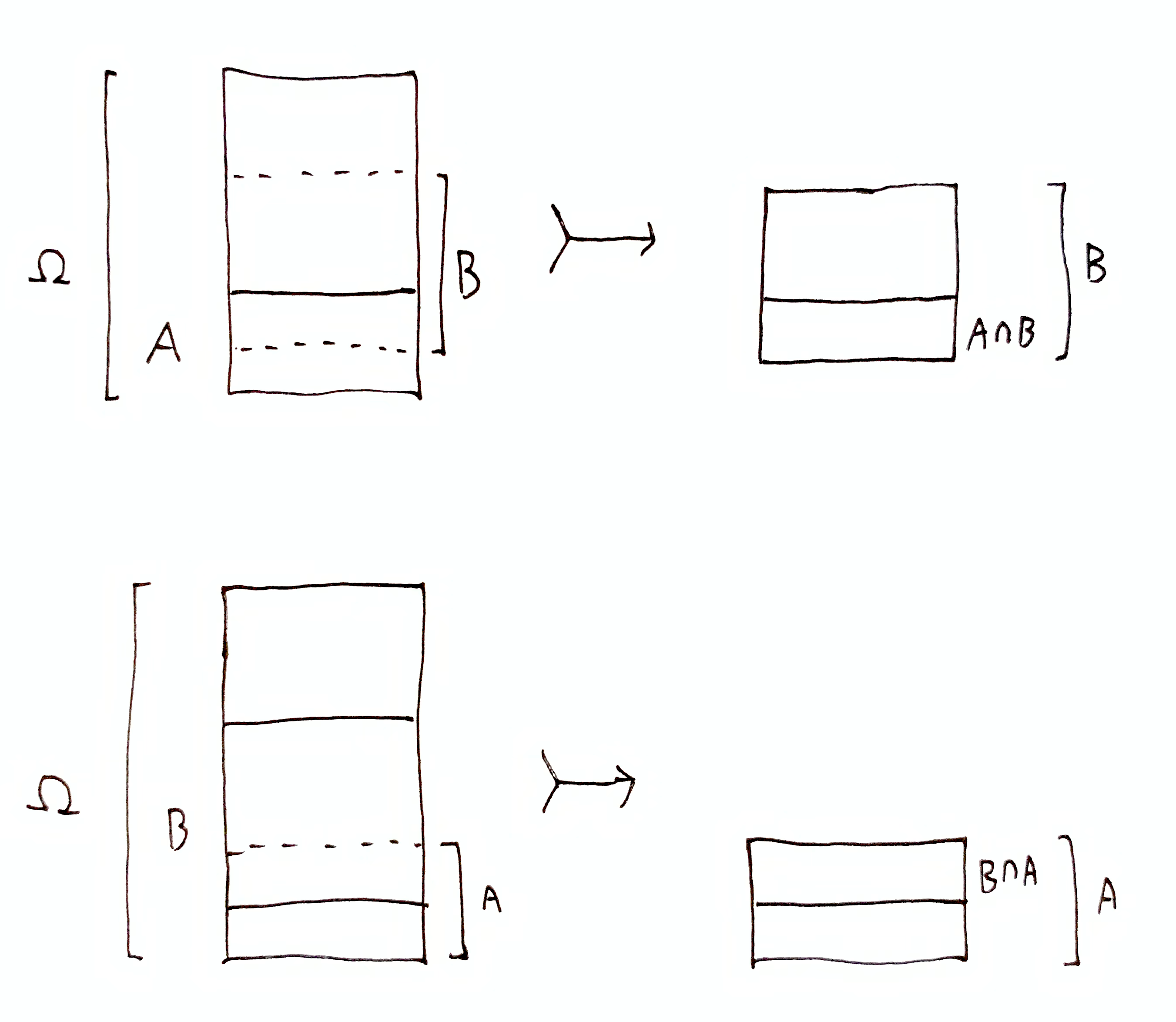
\begin{aligned}
h_\H(A \mid B) &\df h_\H(A\cap B) - h_\H(B) \\
&= -\lg\par{\frac{\abs{A \cap B}}{\abs{B}}} \\
&= h_B(A\cap B)\,.
\end{aligned}
$$
So $h_\H(\dom{\H}{10} \mid \dom{\H}{1}) = h_\H(\dom{\H}{10}) - h_\H(\dom{\H}{1}) \approx 1.415 - 0.415 = 1$. Conditional information gain is just the information gain starting from a different hypothesis set, so $h_\H(\dom{\H}{10} \mid \dom{\H}{1}) = h_{\dom{\H}{1}}(\dom{\H}{10}) = -\lg(3/6) = 1$, which is the number of halvings it takes to get from $\dom{\H}{1}$ to $\dom{\H}{10}$.
The agent would like $h(\dom{\H}{x})$ to be maximized given a pre-defined $\H$, but the agent may not have any control over this quantity, unless the agent can take actions that affect what data $x$ it observes. However, if the agent gets to choose $\H$, then would the agent choose a very small set to begin with so that it does not need to be narrowed down very much?
There is a problem. Take again as an example the rigid agent: $\H = \set{0000000000\dots}$. If only $0$s are ever observed, then this is a great hypothesis set, because the agent will be maximally certain about its prediction of future $0$s, and the agent will be right. But suppose the agent is wrong, e.g. the agent observes data $x = 001$. Then $\dom{\H}{001} = \set{}$ is the empty set. The agent can no longer make any prediction! If we quantify this narrowing-down, we get
$$
h_\H(\dom{\H}{001}) = -\lg\par{\frac{0}{1}} = \infty\,.
$$
We’ve maximized the amount of narrowing-down - it’s infinite. But at the same time this defeats the actual goal of being maximally certain about predictions. Having an empty hypothesis set is a degenerate state. Clearly, too much information gain is bad. Is there an ideal trade-off? That is a question I hope to explore in a future post (unpublished: ).
Compound hypotheses
Consider the following hypothesis set:
$$
\begin{aligned}
\H = \{&0000000000\dots,
\\&0100000000\dots,
\\&0010000000\dots,
\\&0110000000\dots,
\\&1001111111\dots,
\\&1101111111\dots,
\\&1011111111\dots,
\\&1111111111\dots\}
\end{aligned}
$$
The first symbol in these sequences fully determines the long-run behavior of the sequences, i.e. sequences starting with 0 end with 0s, and sequences starting with 1 end with 1s. However, the 2nd and 3rd symbols are not determined by the 1st. Perhaps it would make sense to not care about predicting them. In that case, we are not so interested in narrowing down $\H$ to one sequence, as we are in narrowing down $\H$ into a particular long-run pattern.
$\newcommand{\h}{\mc{H}}$We can formally represent what we care about and don’t care about predicting, by partitioning $\H$. In this example, suppose we make the following partition:
$$
\begin{aligned}
\mf{H} = \set{\h_1, \h_2} = \{
\{&0000000000\dots,
\\&0100000000\dots,
\\&0010000000\dots,
\\&0110000000\dots\},
\\\{&1001111111\dots,
\\&1101111111\dots,
\\&1011111111\dots,
\\&1111111111\dots\}\}
\end{aligned}
$$
$\h_1$ contains only sequences ending in 0s, and $\h_2$ contains only sequences ending in 1s.
In general, for a partition $\mf{H}$ of $\H$, call each $\h\in\mf{H}$ a compound hypothesis, indicating that its a set of primitive hypotheses (data continuations). As we shall see, compound hypotheses correspond closely to the hypotheses-as-data-distributions formulation which we saw in Deconstructing Bayesian Inference.
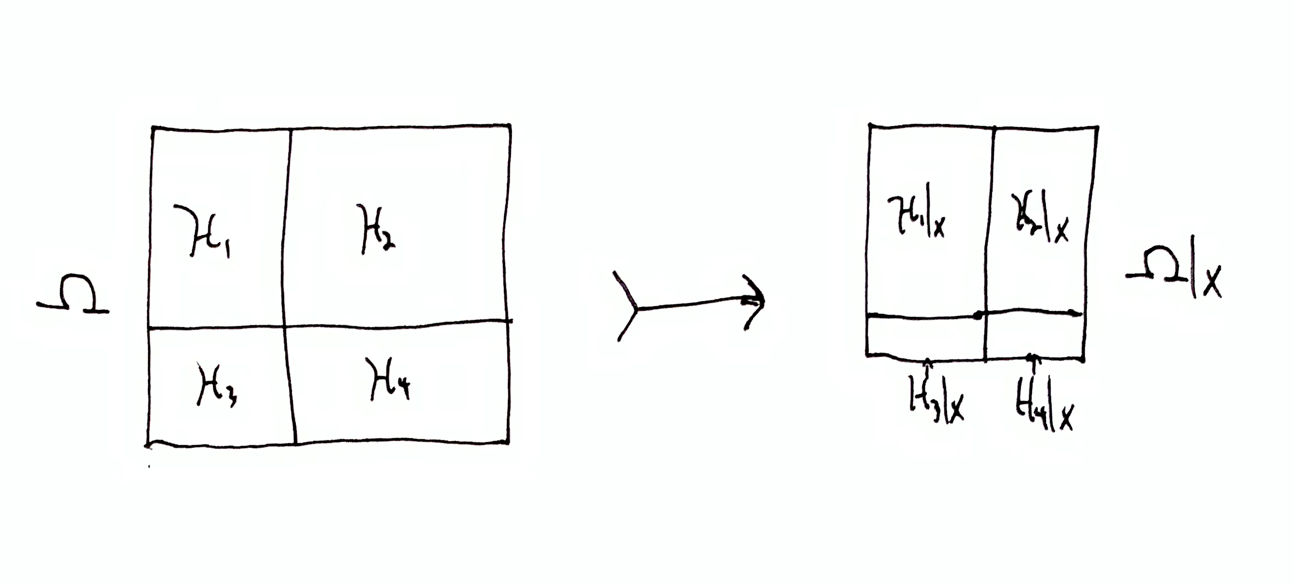
For some partition $\mf{H}$ of $\H$, let $\dom{\mf{H}}{x} = \set{\dom{\h}{x} \mid \h \in \mf{H}}$ be the partition of $\dom{\H}{x}$ consisting of the parts in $\mf{H}$ which have each been conditionalized on $x$ (narrowed down to the sequences starting with $x$).
In our example, $\dom{\mf{H}}{0} = \set{\h_1, \set{}}$ and $\dom{\mf{H}}{1} = \set{\set{}, \h_2}$. Let’s consider empty compound hypotheses to be eliminated. Then in either scenario, observing just the 1st symbol narrows down $\mf{H}$ to exactly one compound hypothesis, analogous to our original goal of narrowing down $\H$ to one hypothesis. The remaining compound hypothesis (either $\h_1$ or $\h_2$) is uncertain about what the 2nd and 3rd symbols will be, but certain about all symbols after that.
Defining Information
Let $\H \subseteq \X^\infty$ be a hypothesis set and $\o\in\X^\infty$ be the true data sequence, i.e. the data sequence that will be observed. Let $\mc{O}\subseteq\H$ be some subset of $\H$ containing $\o$. I define information as a tuple of the form $(\H, \mc{O})$, which specifies a set of possibilities and a narrowed down subset of remaining possibilities. The information $(\H, \mc{O})$ represents the knowledge that $\o\in\mc{O}$ (and equivalently that $\o\notin\H\setminus\mc{O}$). This definition allows us to separate the issue of quantifying information with specifying information. Quantity of information may depend on an arbitrary choice of measure, whereas the information itself is what we often care about.
Below I will use the notation
$$
\H \tr \mc{O} \df (\H, \mc{O})\,,
$$
which can be read as “$\H$ is narrowed down to $\mc{O}$.” This arrow-notation represents information gain, which is equivalent to having the knowledge that $\o\in\mc{O}$ and $\o\notin\H\setminus\mc{O}$. The information gain $\H \tr \mc{O}$ is quantified by $h_\H(\mc{O})$.
Some special cases:
- $(\O, \set{\o})$ is called total information.
- $(\O, \mc{O})$ where $\o\in\mc{O}$ and $\mc{O}\setminus\set{\o}$ is non-empty is called partial information.
- $(\O, \emptyset)$ is called contradictory information
- $(\O, \O)$ is called trivial information.
Information Gain
Earlier, agent’s goal was to gain maximum prediction certainty by narrowing down $\H$ as much as possible. Now with partition $\mf{H}$, the agent’s goal is to narrow down $\mf{H}$ as much as possible, ideally reducing all of the parts but one to empty sets. However, if no compound hypothesis $\dom{\h}{x}\in\dom{\mf{H}}{x}$ is empty, is there still a sense in which the agent narrowed its compound hypotheses down? This question can be answered by considering information gain quantities.
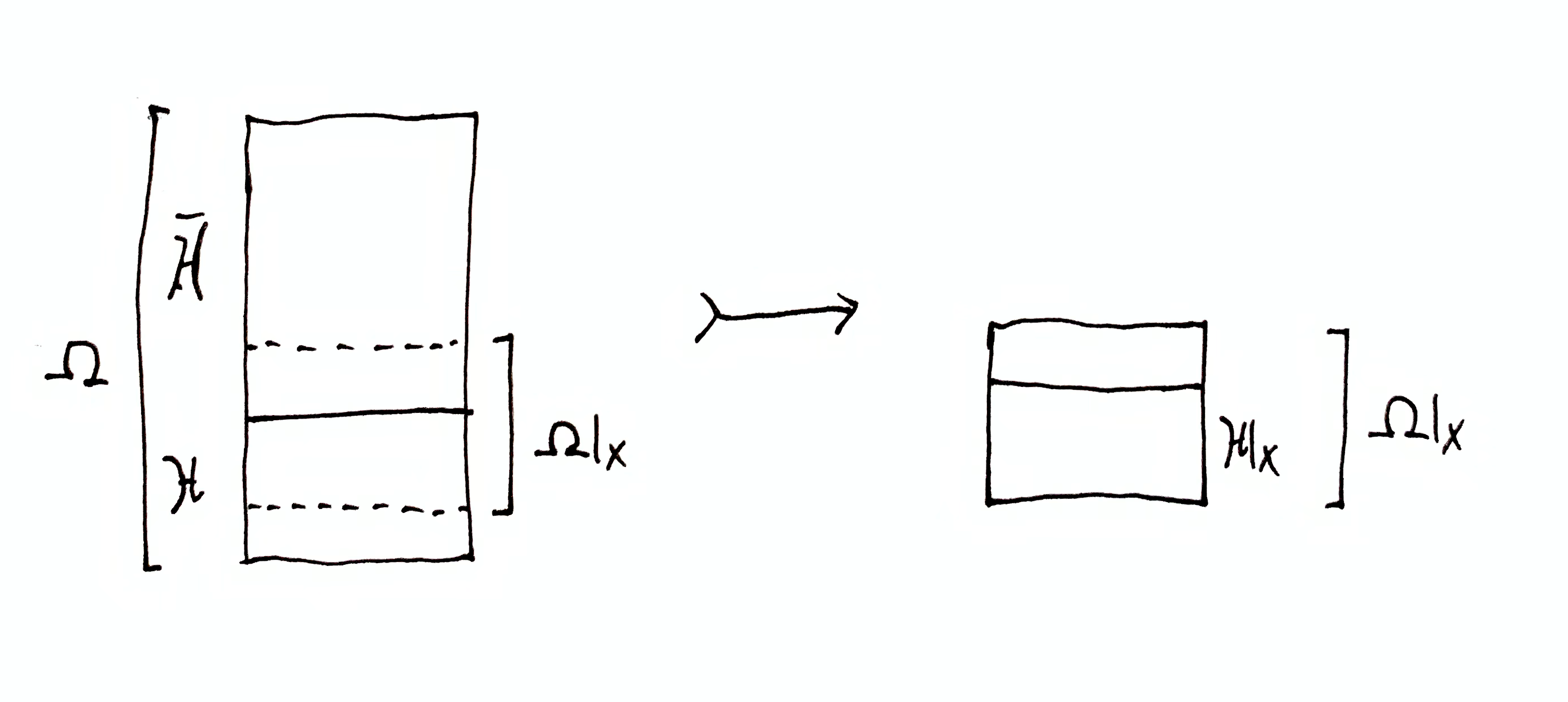
$\H \tr \dom{\H}{x}$ is the total information gained, and is quantified by $h_\H(\dom{\H}{x})$. This is the number of halvings the hypothesis set $\H$ is reduced by due to observing $x$. This quantity does not depend on the choice of partition $\mf{H}$.
$\h \tr \dom{\h}{x}$ is the information gained within compound hypothesis $\h \in \mf{H}$, and is quantified by $h_\H(\dom{\h}{x} \mid \h) = h_\h(\dom{\h}{x})$. This is the information gained where $\h$ is treated as its own hypothesis set. This quantity only depends on the given $\h$, and not the other parts in $\mf{H}$. For each $\h\in\mf{H}$ there is an information gain $\h \tr \dom{\h}{x}$. Since we are considering $\h$ to be a set of sequences that the agent doesn’t care about distinguishing, reductions in $\h$ are essentially wasted information gain. If we regard variation of sequences within $\h$ to be noise, then this quantity measures information gained about that noise.
Let $\o\in\H$ be the full data sequence, of which only a finite prefix $x \sqsubset \o$ has been observed. Call $\o$ the true hypothesis. Likewise, for partition $\mf{H}$ there is exactly one compound hypothesis $\h\in\mf{H}$ containing $\o$. Call this the true compound hypothesis.
Does observing $x$ tell the agent anything about which compound hypothesis $\h\in\mf{H}$ is true (contains $\o$)? Consider first the amount of information gain needed to reach certainty: $\H\tr\h$, i.e. reduce all but one compound hypotheses to the empty set (again, we don’t care about the size of the remaining compound hypothesis). This is quantified by $h_\H(\h)$. When $x$ is observed, $\H$ becomes $\dom{\H}{x}$ and $\h$ becomes $\dom{\h}{x}$. At that point, the information gain needed to achieve certainty that the same compound hypothesis true is $\dom{\H}{x}\tr\dom{\h}{x}$, quantified by $h_{\dom{\H}{x}}(\dom{\h}{x})$.
We haven’t achieved compound hypothesis certainty, but the quantity of information gain needed to do so has changed:
$$
\D_x\up{\h} = h_\H(\h) - h_{\dom{\H}{x}}(\dom{\h}{x})\,.
$$
Let’s confirm that the sign is correct. If $h_{\dom{\H}{x}}(\dom{\h}{x}) > h_\H(\h)$ then we need more bits to achieve $\dom{\H}{x}\tr\dom{\h}{x}$ than to achieve $\H\tr\h$, i.e. the task of narrowing down to this compound hypothesis has gotten harder. In that case, $\D_x\up{\h}$ is negative. If, on the other hand, $h_\H(\h) > h_{\dom{\H}{x}}(\dom{\h}{x})$ then this compound hypothesis has become a larger portion of the remaining $\dom{\H}{x}$ than it was before observing $x$, so the task of narrowing down to this compound hypothesis has gotten easier. In that case, $\D_x\up{\h}$ is positive.
Note that $\D_x\up{\h}$ is upper bounded. If the agent has succeeded in ruling out all other compound hypotheses so that $\dom{\h}{x} = \dom{\H}{x}$, then $h_{\dom{\H}{x}}(\dom{\h}{x}) = 0$ and $\D_x\up{\h} = h_\H(\h)$, which is the maximum amount of information that can be gained about whether $\h$ is true.
If $\h$ is known to be false, i.e. $\dom{\h}{x} = \set{}$, then $h_{\dom{\H}{x}}(\dom{\h}{x}) = \infty$ and so $\D_x\up{\h} = -\infty$. Thus $\D_x\up{\h}$ is not lower bounded, i.e. there is a maximum amount of information to be gained about whether a compound hypothesis is true, but an infinite amount of information to lose. For example, if $\h$ is true but $x$ is very misleading, then $\D_x\up{\h}$ will be very negative. In the long run, if the agent observes enough data, $\o_{1:n}$ for large $n$, then $\D_{\o_{1:n}}\up{\h}$ will go up and eventually converge to $h_\H(\h)$. The misleading initial data caused the agent to lose information, in the sense that even more information needs to be gained to achieve the same certainty that $\h$ is true.
Also note that $\D_x\up{\h}$ is a total change given the entire data sequence $x$. We can also quantify the change due to a single timestep $x_n$:
$$
\D_{x_n}\up{\dom{\h}{x_{<n}}} = h_{\dom{\H}{x_{<n}}}(\dom{\h}{x_{<n}}) - h_{\dom{\H}{x_{1:n}}}(\dom{\h}{x_{1:n}})\,.
$$
Then the total change is the sum of changes for each timestep:
$$
\D_x\up{\h} = \sum_{i=1}^\abs{x} \D_{x_i}\up{\dom{\h}{x_{<i}}}\,.
$$
It may even be of some interest to plot incremental information gains over time for each compound hypothesis $\h$. What we will observe is that in the long run is that $\D_x\up{\h}$ asymptotically converges to $h_\H(\h)$ for the true compound hypothesis $\h$, and the incremental change $\D_{x_n}\up{\dom{\h}{x_{<n}}}$ gets smaller and smaller over time for that same $\h$. Meanwhile, for all other compound hypotheses $\h'$ (the false ones), $\D_x\up{\h'}$ diverges to $-\infty$ and the incremental change $\D_{x_n}\up{\dom{\h'}{x_{<n}}}$ goes negative and grows larger and larger in magnitude. For “misleading” data, the short-run behavior of these plots may be oscillatory before long-run behavior takes over.
Useful Identities
Doing some algebraic manipulation, we get:
$$
\begin{aligned}
\D_x\up{\h} &= h_\H(\h) - h_{\dom{\H}{x}}(\dom{\h}{x}) \\
&= -\lg\par{\frac{\abs{\h}}{\abs{\H}}} + \lg\par{\frac{\abs{\dom{\h}{x}}}{\abs{\dom{\H}{x}}}} \\
&= \lg\par{\frac{\abs{\dom{\h}{x}}/\abs{\dom{\H}{x}}}{\abs{\h}/\abs{\H}}} \\
&= \lg\par{\frac{f_x\up{\h}}{f\up{\h}}}\,,
\end{aligned}
$$
where $f\up{\h} = \abs{\h}/\abs{\H}$ is the fraction of predictions that $\h$ takes up, and $f_x\up{\h} = \abs{\dom{\h}{x}}/\abs{\dom{\H}{x}}$ is that fraction after $x$ is observed. This gives us an interpretation for the quantity $\D_x\up{\h}$: the number of doublings it takes to go from $f\up{\h}$ to $f_x\up{\h}$. E.g. if $\h$ is a quarter the size of $\H$ and $\dom{\h}{x}$ is half the size of $\dom{\H}{x}$, then $\D_x\up{\h} = \lg\frac{1/2}{1/4} = \lg 2 = 1$. That means the agent has one less bit to gain about whether $\dom{\h}{x}$ is true, and has in that sense gained one bit of information.
Doing even more algebra, we get another useful identity:
$$
\begin{aligned}
\D_x\up{\h} &= \lg\par{\frac{\abs{\dom{\h}{x}}/\abs{\dom{\H}{x}}}{\abs{\h}/\abs{\H}}} \\
&= -\lg\par{\frac{\abs{\dom{\H}{x}}}{\abs{\H}}} + \lg\par{\frac{\abs{\dom{\h}{x}}}{\abs{\h}}} \\
&= h_\H(\dom{\H}{x}) - h_\h(\dom{\h}{x})
\end{aligned}
$$
Thus, $h_\H(\dom{\H}{x}) = h_\h(\dom{\h}{x}) + \D_x\up{\h}$, for all $\h\in\mf{H}$. That is to say, the total information gain $h_\H(\dom{\H}{x})$ can be decomposed as the sum of information gained within a given compound hypothesis $\h$ (information gained about noise, i.e. what we don’t care about predicting), plus the information gained about whether $\h$ is true. Total info gain $h_\H(\dom{\H}{x})$ decomposes similarly for every $\h\in\mf{H}$.
Other Information Quantities
See my primer to Shannon’s information theory for more intuition about the interpretation of these quantities, and specifically the sections on
mutual information and entropy.
For sets $A,B\subseteq\H$, the quantity $i_\H(A, B)$ is called the pointwise mutual information (PMI) between $A$ and $B$, defined by
$$
\begin{aligned}
i_\H(A,B) &\df h_\H(A) - h_\O(A \mid B) \\
&= -\lg\par{\frac{\abs{A}}{\abs{\H}}} + \lg\par{\frac{\abs{A\cap B}}{\abs{B}}} \\
&= \lg\par{\frac{\abs{A\cap B}}{\abs{A}\abs{B}}\abs{\H}} \\
&= \lg\par{\frac{\abs{A\cap B}}{\abs{A}\abs{B}}} - \lg\par{\frac{1}{\abs{\H}}}\,.
\end{aligned}
$$
Note that PMI is symmetric, so $i_\H(A, B) = i_\H(B, A)$.
Notice that $\D_x\up{\h} = i_\H(\h, \dom{\H}{x})$. Using our intuition about narrowing down compound hypotheses from before, we can interpret the meaning of $i_\H(A, B)$ in general.
Let
$$
\frac{\H \tr \H'}{U \tr U'}
$$
denote the statement “$\H$ is narrowed down to $\H'$ while $U$ is narrowed down to $U'$”, with the assumption that $U \subseteq \H$ and $U'\subseteq\H'$. So the idea of gaining information about whether compound hypothesis $\h$ is true can be written succinctly as $\frac{\H \tr \dom{\H}{x}}{\h \tr \dom{\h}{x}}$.
In general, $i_\H(A, B)$ quantifies $\frac{\H \tr B}{A \tr (A \cap B)}$, and is the number of doublings achieved from fraction $f = \abs{A}/\abs{\H}$ to fraction $f'=\abs{A\cap B}/\abs{B}$, i.e. $\lg(f'/f)$.
Entropy
It is useful to have a single quantity representing the state of $\dom{\mf{H}}{x}$.
Let $\mf{A}$ be some partition of $\H$. Define entropy
$$
\mb{H}(\mf{A}) \df \sum_{A\in\mf{A}} \frac{\abs{A}}{\abs{\H}} h_\H(A)\,.
$$
This quantity doesn’t require $\O$ to be explicitly specified because it determined by the argument, i.e. $\O = \bigcup \mf{A}$.
Let $\mf{H}$ be a compound hypothesis set. Then $\mb{H}(\mf{H})$ quantifies roughly how much of a difference there is in information that can be gained about whether each compound hypothesis $\h\in\mf{H}$ is true. Specifically, it is the expected information gain across $\mf{H}$, though expectations don’t have the same meaning here because these “probabilities” don’t denote randomness. $\mb{H}(\mf{H})$ is maximized if $h_\H(\h) = h_\H(\h')$ for all $\h,\h'\in\mf{H}$, and $\mb{H}(\mf{H})$ is 0 if one $\h\in\mf{H}$ is non-empty while all other compound hypotheses are empty. If we observe $x$, then high $\mb{H}(\dom{\mf{H}}{x})$ indicates high uncertainty about which compound hypothesis is true, and small $\mb{H}(\dom{\mf{H}}{x})$ indicates high certainty about which compound hypothesis is true.
Mutual Information
Let $\mf{A}$ and $\mf{B}$ be partitions of $\H$. Define mutual information (MI)
$$
\mb{I}(\mf{A}, \mf{B}) \df \sum_{A\in\mf{A}}\sum_{B\in\mf{B}} \frac{\abs{A\cap B}}{\abs{\H}} i_\H(A, B)\,.
$$
This is the expected pointwise mutual information between the two partitions, which quantifies roughly how much redundancy there is between them.
MI plays the following role in Bayesian information gain: Let $\mf{X}_n = \set{\dom{\H}{x} \mid x\in\X^n}$ be the partition of $\H$ consisting of all possible conditionalizations $\dom{\H}{x}$ for each possible length-$n$ data sequence $x\in\X^n$. Then $\mb{I}(\mf{H}, \mf{X}_n)$ quantifies how much information could be gained (in expectation) about which compound hypothesis is true given a (not yet observed) length-$n$ data sequence. If MI is minimized, $\mb{I}(\mf{H}, \mf{X}_n)=0$, then we expect that $\D_x\up{\h} = i_\H(\h, \dom{\H}{x})=0$ for $\h\in\mf{H}$ and $\dom{\H}{x}\in\mf{X}_n$. This would indicate that the partitions $\mf{H}$ and $\mf{X}_n$ are orthogonal, in a sense. On the other hand, MI is maximized when $\mb{I}(\mf{H}, \mf{X}_n)=\min\set{\mb{H}(\mf{H}), \mb{H}(\mf{X}_n)}$, and indicates that each $x\in\X^n$ will narrow down some $\h\in\mf{H}$ to empty sets (with either one remaining compound hypothesis which is narrowed down, or multiple remaining compound hypotheses which are not narrowed down at all), i.e. the partitions are parallel, in a sense.
Infinite possibilities
In practice agents would want to have a large enough hypothesis set to be able to make predictions in all circumstances. That is to say, given any finite observation $x\in\X^*$, it is desirable for at least one sequence $\o\in\H$ to begin with $x$, denoted $x \sqsubset \o$. Then, $\dom{\H}{x}$ is non-empty for all $x$ and so the agent always has at least one prediction to make.
Clearly such an $\H$ cannot be finite because $\X^*$ is infinite, i.e. there is at least one $\o\in\H$ for every $x\in\X^*$ (Simple proof: Suppose $\H$ were finite. Construct finite $x$ s.t. $x\not\sqsubset\o$ for all $\o\in\H$). (Note that such an $\H$ need not be equal to $\X^\infty$. For example, $\H = \set{x`00000\dots \mid x\in\X^*}$ where $x`00000\dots$ is $x$ appended with infinite $0$s. This $\H$ does not include sequences with other limiting behavior, e.g. the binary digits of Pi.)
However, $\H$ can be too big. Suppose $\H=\X^\infty$. Then $\dom{\H}{x} = \X^\infty$ for all $x\in\X^*$. This hypothesis set can never be narrowed down to anything, i.e. there is never information gain. An agent with this hypothesis set remains maximally uncertain always, and so it is not useful.
Even if $\H$ is a strict subset of $\X^\infty$ but contains every finite data sequence (so that $\dom{\H}{x}$ is non-empty for all $x$), it’s usefulness is still dubious. In general $\abs{\dom{\H}{x}}=\infty$ for all $x$ (the cardinality of $\dom{\H}{x}$ is always infinite; disregarding different sizes of infinity), so we cannot compare to what extent we’ve narrowed down $\H$ further by observing $x$ rather than $y$. That is to say, $\abs{\dom{\H}{x}}/\abs{\H} = \infty/\infty$ is indeterminate. Furthermore, $\dom{\H}{x}$ will contain every finite data sequence starting with $x$, so there is no tangible sense in which the agent’s predictions at finite time are narrowed down.
The problem of measuring narrowing-down of infinite possibility sets is resolved by choosing a measure $\mu$ on $\H$. However a new problem arises: how to choose $\mu$. My purpose in presenting Bayesian information theory as narrowing down possibility spaces is to give meaning to probability values. Now, we’ve reintroduced an arbitrary measure $\mu$.
There is a sort of middle ground that also serves as a bridge between the usual probabilistic conception of Bayesian inference I introduced in Deconstructing Bayesian Inference and the hypothesis set conception, via algorithmic information theory.
Algorithmic Randomness
In Deconstructing Bayesian Inference, I defined Bayesian inference as a manipulation of probability measures on $\X^\infty$. Given a set $\M$ of measures $\mu$ on $\X^\infty$, and a prior $p$ on $\M$, what is the corresponding “possibility space narrowing-down” perspective?
I supposed that hypothesis probabilities $\mu(\o_{1:n})$ for $\mu\in\M$ represented irreducible uncertainty about the world, whereas subjective probabilities $p(\o_{1:n})$ represented a mixture of reducible and irreducible uncertainty, where knowing which hypothesis $\mu$ is true maximally reduces your uncertainty.
I also introduced a distinction between randomness and non-determinism. Randomness can be defined as incompressibility, and non-determinism refers to the output of a mathematical construct (such as a function) being not uniquely determined by givens (such as an input). Probabilities can measure both, which can lead to confusion.
Let’s suppose here that hypothesis probabilities always measure randomness. Assuming $\mu\in\M$ is computable, we can precisely define what it means for an infinite sequence $\o\in\X^\infty$ to “look like” a typical sequence randomly drawn from $\mu$. Call such “typical looking” sequences $\mu$-typical (or $\mu$-random). Formally, $\o\in\X^\infty$ is $\mu$-typical iff the optimal compression rate of $\o$ (via monotone algorithmic complexity $Km$) is achieved with arithmetic coding using $\mu$. (See Li & Vitányi, 3rd edition, theorem 4.5.3 on page 318, which states, $\sup_n\left\{\lg(1/\mu(\o_{1:n})) - Km(\o_{1:n})\right\} < \infty$.)
Let $\h\up{\mu}\subseteq\X^\infty$ be the set of all infinite sequences which are $\mu$-typical, called the $\mu$-typical set. The $\mu$-probability of drawing a $\mu$-typical sequence is 1, i.e. $\mu(\h\up{\mu})=1$, and the $\mu$-probability of drawing a $\mu$-atypical sequence is 0. You can think of $\h\up{\mu}$ as $\X^\infty$ with a $\mu$-measure 0 subset subtracted from it (specifically $\h\up{\mu}$ is the smallest constructable $\mu$-measure 1 subset of $\X^\infty$).
The prior $p$ on $\M$ induces a subjective data distribution: $p(\o_{1:n}) = \sum_{\mu\in\M} p(\mu)\mu(\o_{1:n})$. So long as $p$ is computable, there is a $p$-typical set $\h\up{p}$.
Let $\H = \h\up{p}$ and $\mf{H} = \set{\h\up{\mu} \mid \mu\in\M}$, where $\H$ is an agent’s hypothesis set (set of sequence predictions) and $\mf{H}$ is a set of compound hypotheses, where $\bigcup \mf{H} = \H$. I’m dropping the requirement that $\mf{H}$ be a proper partition of $\O$ (i.e. all $\h\in\mf{H}$ are mutually disjoint), in which case we call $\mf{H}$ a cover of $\O$.
Now, Bayesian inference with hypothesis set (of measures) $\M$ and prior $p$, and Shannon quantities using these measures, corresponds to Bayesian inference with $\H$ and $\mf{H}$ as I outlined above. The restriction $\dom{\H}{x}$ is the typical set for the conditional measure $p(\cdot \mid x)$, and likewise for $\h\up{\mu}\in\mf{H}$, the restriction $\dom{\h\up{\mu}}{x}$ is the typical set for the conditional measure $\mu(\cdot \mid x)$.
The prior $p(\mu)$ is simply the relative size of $\h\up{\mu}$ within $\H$, given by $p(\h\up{\mu})$. The prior encodes how much information we would gain if all other hypotheses were ruled out: $\H\tr\h\up{\mu}$, quantified by $h_p(\h\up{\mu}) = -\lg p(\h\up{\mu})$.
The posterior $p(\mu\mid x)$ is simply the relative size of $\dom{\h\up{\mu}}{x}$ within $\dom{\H}{x}$, given by $p(\dom{\h\up{\mu}}{x}) = p(\h\up{\mu} \cap \dom{\H}{x})$. The posterior encodes how much information we would gain if all other hypotheses were ruled out (after observing $x$): $\dom{\H}{x}\tr\dom{\h\up{\mu}}{x}$, quantified by $h_p(\h\up{\mu} \mid \dom{\H}{x}) = -\lg p(\dom{\h\up{\mu}}{x})/p(\dom{\H}{x})$.
Furthermore, $\H\tr\dom{\H}{x}$ is quantified by $h_p(\dom{\H}{x}) = -\lg p(\dom{\H}{x}) = -\lg p(x)$, and $\h\up{\mu}\tr\dom{\h\up{\mu}}{x}$ is quantified by $h_\mu(\dom{\h\up{\mu}}{x}) = -\lg \mu(\dom{\h\up{\mu}}{x}) = -\lg \mu(x)$.
The mysterious “information gained about whether hypothesis $\mu$ is true” becomes $\frac{\H \tr \dom{\H}{x}}{\h\up{\mu} \tr \dom{\h\up{\mu}}{x}}$, quantified by $i_p(\h\up{\mu}, \dom{\H}{x}) = \lg\frac{p(\dom{\h\up{\mu}}{x})}{p(\h\up{\mu})p(\dom{\H}{x})} = \lg\frac{p(\mu,x)}{p(\mu)p(x)}$ which is the pointwise mutual information between hypothesis $\mu$ and data $x$.
Finally, the information gained about which hypothesis is true is summarized by the quantity
$$\mb{I}_p(\mf{H}, \mf{X}_\abs{x}) = \sum_{\h\up{\mu}\in\mf{H}}\sum_{\dom{\H}{x}} \mu(\dom{\h}{x}) i_p(\h\up{\mu}, \dom{\H}{x}) = \mb{E}_p\left[i(H,X_{1:\abs{x}})\right] = I(H, X_{1:\abs{x}})\,,$$
where $H$ is the random variable corresponding to choice of hypothesis $\mu$ sampled from $p(\mu)$ and $X_{1:\abs{x}}$ is the random variable corresponding to choice of length-$\abs{x}$ data sampled from $p(x)$. This quantity is sometimes called Bayesian surprise (see ref 1 and ref 2), though more commonly “surprise” refers to the total info gain $h_\mu(\dom{\H}{x})$ (ref 1, ref 2).
Posterior consistency
When $\mf{H}$ is a strict partition, this is a special (and desirable) case in Bayesian inference, called posterior consistency. Informally, posterior consistency is when posterior probabilities converge to one-hot (or Dirac delta) distributions (almost surely). Posterior consistency is a property of a particular set of hypotheses $\M$, and is invariant to prior probabilities (assuming suppose on $\M$).
If $\M$ has the posterior consistency property, then the corresponding $\mf{H}$ will be nearly a partition, where $\mu(\h\up{\mu}\cap\h\up{\nu}))=\nu(\h\up{\mu}\cap\h\up{\nu}))=0$, for $\mu,\nu\in\M$.
Posterior inconsistency in $\M$ corresponds to $\mf{H}$ which has overlapping compound hypotheses (of non-zero measure).
Why do we want $\mf{H}$ to be a partition? So then information gained about one hypothesis $\mu$, corresponding to compound hypothesis $\h\up{\mu}$, necessarily implies information loss about all other hypotheses. If compound hypotheses overlap, then you can become more certain about multiple hypotheses at the same time, and in the infinite data limit, many hypotheses may remain (and we have not achieved our goal of prediction certainty by narrowing down to one hypothesis).
Posterior convergence
For any typical set $\h\up{\mu}$, there are actually infinitely many computable measures with the same typical set. Why is that? For any $\mu$, a new measure $\mu'$ can be constructed that assigns different probabilities than $\mu$ to finite sequences, e.g. $\mu'(\o_{1:n}) \neq \mu(\o_{1:n})$, while preserving the limiting compression rates:
$$\lim_{n\to\infty} \frac{1}{n}\lg\par{\frac{1}{\mu(\o_{1:n})}} = \lim_{n\to\infty} \frac{1}{n}\lg\par{\frac{1}{\mu'(\o_{1:n})}}$$
A difference in probabilities of finite sequence $\o_{1:n}$ corresponds to a constant offset in compression length (according to Shannon):
$$\abs{\lg\par{\frac{1}{\mu(\o_{1:n})}} - \lg\par{\frac{1}{\mu'(\o_{1:n})}}} = C < \infty$$
Any finite difference becomes negligible as $n\to\infty$. $\mu$ is said to have posterior convergence to $\mu'$.
This is a strange predicament, because it implies that there are infinitely many probability measures that essentially encode the same randomness. That is to say, the measurement of randomness of finite sequences is not uniquely determined. This actually falls in line with the results of algorithmic information theory, where optimal compression length (Kolmogorov complexity) depends on choice of programming language (universal Turing machine), and is also arbitrary for that reason.
It is the infinite sequences which have a unique quantity of randomness, in a sense. Non-computable infinite sequences have a compressed length that is also infinite, but often a finite compression rate: $\limsup_{n\to\infty}\frac{Km(\o_{1:n})}{n}$. Moreover, $\o$ has a unique limiting data posterior, i.e.
$$
\lim_{n\to\infty} \mu(\o_n \mid \o_{<n}) - \mu'(\o_n \mid \o_{<n}) = 0\,,
$$
(almost surely), for any two measures $\mu$ and $\mu'$ which have the same typical set $\h\up{\mu}$. Solomonoff’s universal data distribution $\xi$ (the mixture of all semicomputable semimeasures, see Deconstructing Bayesian Inference) has posterior convergence to all such $\mu$. In fact, Solomonoff’s mixture can be used as a test for whether $\o$ is $\mu$-typical by observing if $\lim_{n\to\infty} \xi(\o_n \mid \o_{<n}) - \mu(\o_n \mid \o_{<n}) = 0$ (almost surely).
The takeaway here is that if compound hypothesis $\h$ is the typical set for some measure $\mu$, then if we don’t specify any particular measure, the limiting information gain $h_\H(\dom{\h}{x’y} \mid \dom{\h}{x})$ as $\abs{x}\to\infty$ converges to something unique. So if we have infinite hypothesis sets and don’t want to arbitrarily choose a measure, not all hope is lost.
Shannon Equivalence
I defined the quantities of information above using the set cardinality function $\abs{\cdot}$ to measure the sizes of sets (called the counting measure). In general, the size of a set can be defined with a measure, which is a function from subsets to non-negative real numbers. So a measure $\mu$ on $\H$ has the type signature $\mu : 2^\H \to \mb{R}_{\geq 0}$ (though technically we need to restrict ourselves to measurable subsets of $\H$, see my primer to measure theory for details). Furthermore, if we choose measure $\mu$ s.t. $\mu(\H) = 1$, then $\mu$ is called a probability measure (or a normalized measure). See my primer to probability theory for details.
If we replace $\abs{\cdot}$ with probability measure $\mu(\cdot)$ everywhere in the quantities of information defined above, then we get the usual Shannon definitions:
- $h_\mu(A) = -\lg \mu(A)$
- $h_\mu(A \mid B) = -\lg \par{\frac{\mu(A \cap B)}{\mu(B)}}$
- $i_\mu(A, B) = \lg\par{\frac{\mu(A\cap B)}{\mu(A)\mu(B)}}$
- $\mb{H}_\mu(\mf{A}) = \sum_{A\in\mf{A}} \mu(A) h_\mu(A)$
- $\mb{H}_\mu(\mf{A}\mid B) = \sum_{A\in\mf{A}} \mu(A\mid B) h_\mu(A\mid B)$
- $\mb{H}_\mu(\mf{A}\mid\mf{B}) = -\sum_{A\in\mf{A}}\sum_{B\in\mf{B}} \mu(A\cap B) h_\mu(A\mid B)$
- $\mb{I}_\mu(\mf{A}, \mf{B}) = \sum_{A\in\mf{A}}\sum_{B\in\mf{B}} \mu(A\cap B) i_\mu(A, B)$
where $A,B\subseteq\H$ and $\mf{A},\mf{B}$ are two partitions of $\H$. Note that $\abs{\H}$ disappears because it becomes $\mu(\H) = 1$.
If we don’t use a normalized (probability) measure, i.e. $\mu(\H)$ is anything (except non-zero), then we can also calculate information quantities:
- $h_\mu(A) = -\lg \par{\frac{\mu(A)}{\mu(\H)}}$
- $h_\mu(A \mid B) = -\lg \par{\frac{\mu(A \cap B)}{\mu(B)}}$
- $i_\mu(A, B) = \lg\par{\frac{\mu(A\cap B)\mu(\H)}{\mu(A)\mu(B)}}$
… etc. Though, if $\mu(\H)$ is infinite or not defined (i.e. $\mu$ is not normalizable), then these quantities are not well defined. However, that is alright, since my definition of information is based on the sets of possibilities involved. How those sets are quantified is secondary. That is to say, the intricacies of getting quantification of information to work out don’t bear weight on what information actually is. I am not defining information as its quantity (Shannon information theory could be construed as doing that), and I don’t necessarily require that information gain (and mutual information, etc.) is always quantifiable (its quantity could be undefined or infinite).
Optimal Compression
Now we see that Bayesian information theory is mathematically equivalent to Shannon’s information theory, where a probability measure $\mu$ is used to measure the sizes of hypothesis sets (sets of predictions).
However, what is the connection between narrowing down hypothesis sets and optimal compression? Given probability measure $\mu$ on $\H$, the $\mu$-probability of finite observation $x\in\X^*$ is $\mu(\dom{\H}{x})$. (We can abuse notation and write $\mu(x)$ where $x$ is shorthand for $\dom{\H}{x}$ when given as the argument to $\mu$.) Then is $h_\mu(\dom{\H}{x})$ the optimal compressed length of $x$?
For finite strings, optimal compression isn’t a well defined notion. According to algorithmic information theory, we use the shortest program that outputs $x$ as the compressed representation of $x$, but the length of that shortest program depends on our arbitrary choice of programming language. We can achieve an encoded length of approximately $h_\mu(\dom{\H}{x})$ by using arithmetic coding, with $\mu$ as the provided measure (ignoring the length of the arithmetic decoder program itself).
Shannon’s information theory operates in the domain of random data, and provides optimal code lengths in expectation. In the Bayesian information theory I’ve outlined above, we are not working with randomness, but non-determinism (the agent’s predictions are not uniquely determined). However, as the data length goes to infinity, these two conceptions of probability become intertwined.
Let $\o\in\X^\infty$ be an infinite sequence, and an agent observed the finite prefix $\o_{1:n}$. If the agent has a hypothesis set $\H$ with probability measure $\mu$, the agent can use arithmetic coding w.r.t. $\mu$ to achieve compressed length $-\lg \mu(\o_{1:n})$, and limiting compression rate
$$
\limsup_{n\to\infty} \frac{1}{n}\lg\par{\frac{1}{\mu(\o_{1:n})}}\,.
$$
If $\o$ is $\mu$-typical, than this will be the optimal compression rate achievable (according to algorithmic information theory). However, if $\o$ is not $\mu$-typical then the agent’s compression rate will be worse than the optimum.
Let $\X = \set{0,1}$. For each bit of data $\o_n$, the approximate compressed length of that bit is $-\lg\mu(\o_n \mid \o_{<n})$. So if the agent gains more than 1 bit of information from $\o_n$, arithmetic coding w.r.t. $\mu$ will actually assign more than one bit to $\o_n$ in the compressed representation. If the agent’s info gain remains high in the long run, this “compression” of $\o$ will end up being longer than $\o$ itself (specifically, the compression of $\o_{1:n}$ will be longer than $n$ as $n\to\infty$). This gives us a precise sense about whether the agent is doing a good job at predicting the part of $\o$ that can be predicted: If the agent’s $\mu$-compression rate is better than the length of the data itself then the agent is predicting the data at least better than random.
A mixture distribution can be viewed as a hedge against bad compression. Suppose $\o$ is not $\mu$-typical. If instead of using $\mu$ to predict $\o$, we had a set of distributions $\M$ of which $\mu$ is a member, and we use the mixture $p = \sum_{\nu\in\M} w_\nu \nu$ to predict $\o$. If $\o$ is typical w.r.t. at least one $\nu\in\M$, then $\o$ is also $p$-typical. The difference between using $\nu$ and $p$ to compress $\o$ is
$$
\limsup_{n\to\infty} \lg\par{\frac{1}{p(\o_{1:n})}} - \lg\par{\frac{1}{\nu(\o_{1:n})}} \,,
$$
which is a constant cost in compression length, and becomes negligible in the long run as $n\to\infty$, i.e. the compression rate using $p$ and $\nu$ is the same. So using a mixture to compress $\o$ may incur additional cost (extra bits) initially, in the long run it is no worse than using the “true” hypothesis $\nu$ (there may be more than one “true” hypothesis in $\M$). A good strategy is then to make $\M$ as large as possible. This is the premise behind Solomonoff induction, where $\M$ is the set of all semicomputable semimeasures.