[This is an article, which is something I’ve optimized for readability and transmission of ideas, opposed to notes that are the seed of an idea and something I’ve written quickly.]

I pose the question: Why predict probabilities rather than predicting outcomes without probabilities? I first define Bayesian inference, and then I remove the probabilities involved in multiple passes until there is no probability. Then I examine what the result is, and eventually motivate bringing probabilities back into our predictions.

At any point, feel free to look at the #Use Cases section for examples of Bayesian inference to use as intuition pumps.

$$
\newcommand{\0}{\mathrm{false}}
\newcommand{\1}{\mathrm{true}}
\newcommand{\mb}{\mathbb}
\newcommand{\mc}{\mathcal}
\newcommand{\and}{\wedge}
\newcommand{\or}{\vee}
\newcommand{\a}{\alpha}
\newcommand{\t}{\theta}
\newcommand{\T}{\Theta}
\newcommand{\o}{\omega}
\newcommand{\O}{\Omega}
\newcommand{\x}{\xi}
\newcommand{\z}{\zeta}
\newcommand{\l}{\lambda}
\newcommand{\fa}{\forall}
\newcommand{\ex}{\exists}
\newcommand{\X}{\mc{X}}
\newcommand{\Y}{\mc{Y}}
\newcommand{\Z}{\mc{Z}}
\newcommand{\H}{\mc{H}}
\newcommand{\P}{\mc{P}}
\newcommand{\y}{\psi}
\newcommand{\p}{\phi}
\newcommand{\B}{\mb{B}}
\newcommand{\m}{\times}
\newcommand{\E}{\mb{E}}
\newcommand{\e}{\varepsilon}
\newcommand{\set}[1]{\left\{#1\right\}}
\newcommand{\abs}[1]{\left\lvert#1\right\rvert}
\newcommand{\inv}[1]{{#1}^{-1}}
\newcommand{\ceil}[1]{\left\lceil#1\right\rceil}
$$

Constructing Bayesian Inference

An “agent” here refers to a physical entity that tries to predict the future. An agent can be a robot or a biological organism. Either way, the agent receives a stream of sensory data over the course of its life. The agent’s goal is to predict the future of this stream, in some capacity. Predictions about high-level objects and states of the world are made indirectly by predicting their effect on the sensory stream. That is to say, all prediction can be rolled into predicting the sensory stream. Though the agent may also act to influence the future of its sensory stream, for simplicity, I will consider only prediction and not actions.

Let’s work in discrete time.
Let $\X$ be the set of possible observations at each time-step.
The agent’s sensory stream is a sequence $(x_1, x_2, x_3, \dots) \in \X^\infty$. I’m assuming the sensory stream is infinite, i.e. the agent lives forever. This is not a reasonable assumption but it’s workable. The alternative (that the stream is finite) is more complicated because it requires the agent to predict the end time of its own stream (presumably when it will die).

Let $\o\in\X^\infty$.
$\o_i$ denotes the $i$-th binary value in $\o$.
$\o_{(i_1,i_2,\dots)}$ denotes the sub-sequence of $\o$ indexed by the sequence $(i_1,i_2,\dots)$.
$\o_{i:j} = \o_{(i,i+1,\dots,j-1,j)}$ denotes the slice of $\o$ starting from $i$ and ending at $j$ (inclusive).
$\o_{<i} = \o_{1:i-1}$ denotes the slice up to position $i-1$.
$\o_{\leq i} = \o_{1:i}$ includes $i$.
$\o_{>i} = \o_{i+1:\infty}$ denotes the unbounded slice starting at position $i+1$.

Let $\X^* = \X^0 \cup \X^1 \cup \X^2 \cup \X^3 \cup \dots$ be the union of all finite cartesian products of $\X$, i.e. the set of all finite sequences of any length.
Let $x,y\in\X^*$ be finite sequences.
Denote $\abs{x}$ as the length of $x$.
Denote $x`y = (x_1, \dots, x_\abs{x}, y_1, \dots, y_\abs{y})$ as the sequence concatenation of $x$ and $y$.
Denote $x \sqsubset y$ to mean that $x = y_{1:\abs{x}}$, i.e. $x$ is a prefix of $y$.

Defining A Hypothesis

As the agent gains sensory data, the agent will try to explain that data with various hypotheses. What constitutes a hypothesis is perhaps an open problem in epistemology. I will give the standard idea of “hypothesis” within Bayesian epistemology.

A hypothesis is a probability measure, $\mu$, over all possible sensory streams, $\X^\infty$. That means we can compute the $\mu$-probability of any set of infinite sequences, i.e. $\mu(A)$ for $A \subseteq \X^\infty$. Typically there is a set of hypotheses $\H$ under consideration, i.e. $\H$ is a set of different $\mu$.

For any $\o\in\X^\infty$, the prefix $\o_{1:n}$ is a partial sensory sequence. The marginal $\mu$-probability of $\o_{1:n}$ is $\mu(\Gamma_{\o_{1:n}})$ where $\Gamma_{\o_{1:n}} = \set{\z\in\X^\infty \mid \o_{1:n}\sqsubset\z}$ is the set of all infinite sequences starting with $\o_{1:n}$, called a cylinder set. For notational simplicity, I will write $\mu(x)$ to denote $\mu(\Gamma_{x})$ when $x$ is a finite sequence, so $\mu(\o_{1:n})$ denotes $\mu(\Gamma_{\o_{1:n}})$.

The quantity $\mu(\o_n \mid \o_{<n}) = \mu(\o_{1:n})/\mu(\o_{<n}) = \mu(\o_{1:n})/\mu(\o_{1:n-1})$ is the conditional $\mu$-probability of $\o_n$ given $\o_{<n}$ was already observed.

$\mu$ defined in this way will guarantee that the following holds:

$$
\mu(\o_{<n}) = \int_\X \mu(\o_{<n}`\chi)d\chi\,.
$$

(replace integral with sum for countable $\X$.)

Note that for most $\o\in\X^\infty$,

$$
\lim_{n\to\infty} \mu(\o_{1:n}) = 0\,,
$$

which is similar to how a probability distribution on the real unit interval may assign 0 probability to any particular real number. Here $\o_{1:n}$ acts like an interval, which has probability mass, and the full sequence $\o$ acts like a single point, which does not have probability mass.

A hypothesis $\mu$ ideally represents some primitive way the world might be. We might say a hypothesis probability $\mu(\o_{1:n})$ is objective in some sense. Hypotheses that assign probabilities to outcomes are supposing the universe has inherent randomness that cannot be known before hand (we could also have deterministic hypotheses that assign probabilities of either 0 or 1).

Bayesian inference distinguishes between two kinds of uncertainty: that due to inherent randomness in the universe, and that due to lack of knowledge of the agent. This distinction between kinds of uncertainty may not be precise (and I’m not sure I agree that such a distinction should be made), but this is typically how hypothesis probabilities are conceptually distinguished from subjective data probabilities (which I’ll get to in a moment).

In this framing, the goal of Bayesian inference is to calculate one’s certainty (or uncertainty) that each hypothesis being considered explains the observed data. This kind of uncertainty is represented with probabilities just like irreducible uncertainty, but the former is in principle reducible to certainty. As the agent observes data, these probabilities change, and hence the agent’s uncertainty about each hypothesis changes over time (potentially approaching certainty).

Defining Bayesian Inference

Let $\X^\infty$ be the set of all possible observations (infinite data sequences).
Let $\H$ be a set of hypotheses (probability measures on $\X^\infty$).

I will induce a joint probability distribution on $\H$ and $\X^\infty$.
Let $p(\mu)$ be the prior probability of $\mu\in\H$.
Let $p(\o_{1:n} \mid \mu) = \mu(\o_{1:n})$ be the data probability of $\o_{1:n}$ under hypothesis $\mu$. This is read as, “the probability of data $\o_{1:n}$ given hypothesis $\mu$.” Here, “giving the hypothesis” is equivalent to specifying what data distribution should be used to calculate the probability of $\o_{1:n}$.

$p(\mu,\o_{1:n}) = p(\mu)p(\o_{1:n} \mid \mu) = p(\mu)\mu(\o_{1:n})$ is the joint probability of $\mu$ and $\o_{1:n}$. From here, we can compute any other quantity of interest.

$$p(\o_{1:n}) = \int_\H p(\mu,\o_{1:n})d\mu = \int_\H p(\mu)\mu(\o_{1:n})d\mu$$

is called the subjective (Bayesian) data probability of $\o_{1:n}$ (replace integrals with sums if $\H$ is discrete). $p(\o_{1:n})$ does not condition on a hypothesis, and is the sum/integral over every hypothesis probability $\mu(\o_{1:n})$ weighted by the prior $p(\mu)$. You can think of $p(\o_{1:n})$ as a weighted-average over hypothesis probabilities.

If a hypothesis probability $\mu(\o_{1:n})$ is objective in some sense (a hypothesis represents the way the world actually might be), then a prior probability $p(\mu)$ represents the agent’s state of certainty/uncertainty about $\mu$ being true (how the world actually is). If the agent knew that $\mu$ was the case, then the agent would just use $\mu$ to predict the future sensory data, where $\mu$-probabilities are due to inherent randomness in the data. However, since the agent has uncertainty about which hypothesis is the case, $p(\o_{1:n})$ represents the agent’s total uncertainty about $\o_{1:n}$ occurring, which is a combination of inherent randomness in the data and the agent’s lack of knowledge about which hypothesis is true.

Another quantity of interest:

$$
\begin{aligned}
p(\mu\mid\o_{1:n}) &= p(\mu,\o_{1:n})/p(\o_{1:n}) \\ \\
&= \frac{p(\mu)p(\o_{1:n}\mid\mu)}{p(\o_{1:n})}\\ \\
&= p(\mu)\frac{\mu(\o_{1:n})}{p(\o_{1:n})}
\end{aligned}
$$

is called the hypothesis posterior probability (or more commonly, just “posterior") of hypothesis $\mu$ given data $\o_{1:n}$. This quantity represents the agent’s certainty/uncertainty about hypothesis $\mu$ after observing $\o_{1:n}$. If we are viewing $p(\mu)$ as a weight, then the weight on $\mu$ updates to $p(\mu\mid\o_{1:n})$ when $\o_{1:n}$ is observed. In this sense, the agent updates its knowledge (confidence) about the hypotheses in $\H$ when data is observed. The last equation is a prescription for an update rule on these uncertainty weights on $\mu$, taking the form $w' = \gamma w$, where $\gamma = \mu(\o_{1:n})/p(\o_{1:n})$ is a multiplicative adjustment on the prior weight $w$.

Observing additional data amounts to appending $\o_{n+1:m}$ to $\o_{1:n}$, and the weight on $\mu$ updates again to $p(\mu\mid\o_{1:m})$. This iterative process of observing more data and updating can go on forever, so long as the data space $\X^\infty$ consists of infinite sequences.

As a side note, you should recognize $p(\mu\mid\o_{1:n})=p(\o_{1:n}\mid\mu)p(\mu)/p(\o_{1:n})$ as the classic form of Bayes rule (typically used to explain Bayesian inference). Usually, it is written like this: $p(H \mid D) = p(D \mid H)p(H)/p(D)$, where $H$ is a random variable for hypotheses (often parameter $\Theta$ is used in place of $H$), and $D$ is a random variable for datasets. In my opinion this form hides the sequential nature of Bayesian inference and is pedagogically confusing for that reason.

In general, the agent wants to predict what sensory data will occur after $\o_{\leq n}$ has been observed. For that, we need the data posterior probability

$$
\begin{aligned}
p(\o_{>n} \mid \o_{\leq n}) &= \int_\H p(\mu, \o_{>n} \mid \o_{\leq n})d\mu \\
&= \int_\H p(\o_{>n} \mid \mu, \o_{\leq n})p(\mu\mid\o_{\leq n})d\mu \\
&= \int_\H p(\mu\mid\o_{\leq n})p(\o_{>n} \mid \o_{\leq n},\mu)d\mu \\
&= \int_\H p(\mu\mid\o_{\leq n})\mu(\o_{>n} \mid \o_{\leq n})d\mu \\
&= \int_\H p(\mu)\frac{\mu(\o_{\leq n})}{p(\o_{\leq n})}\mu(\o_{>n} \mid \o_{\leq n})d\mu\,.
\end{aligned}
$$

Like the subjective data probability $p(\o_{\leq n})$, the data posterior probability $p(\o_{>n} \mid \o_{\leq n})$ is subjective, in the sense that it reflects the agent’s uncertainty about the outcome, as well as any irreducible randomness. These two quantities have the same form: $p(\o_{\leq n})$ averages over $p(\mu)\mu(\o_{\leq n})$, and $p(\o_{>n} \mid \o_{\leq n})$ averages over $p(\mu\mid\o_{\leq n})\mu(\o_{>n} \mid \o_{\leq n})$. Either way, $p(\o_{\leq n})$ and $p(\o_{>n} \mid \o_{\leq n})$ are both weighted averages over all hypothesis probabilities, i.e. the inherent randomness of each hypothesis is weighted by the agent’s uncertainty about that hypothesis. The only difference is that the posterior conditions everything on the observed $\o_{\leq n}$.

Deconstructing Bayesian inference

To review, we assumed the agent has a set of hypotheses $\H$, where each hypothesis $\mu\in\H$ is a probability measure on infinite data sequences $\X^\infty$. For partial observation $\o_{1:n}$, each hypothesis assigns probability $\mu(\o_{1:n})$. Putting a prior on $\H$ allows us to compute $p(\o_{1:n})$, which is the “average” $\mu$-probability of $\o_{1:n}$. The resulting distribution $p$ is called the subjective data distribution.

Removing hypotheses

Question: What is the difference between a hypothesis $\mu$ and a subjective data distribution $p$? Do we need hypotheses at all?

They appear to have the same form: $\mu(\o_{1:n})$ vs $p(\o_{1:n})$. Above I gave a hand-wavy interpretational difference between the two. However, it is the case that hypotheses are not strictly necessary for predicting the continuation of a data sequence (equivalent to the singleton hypothesis space $\H = \set{p}$).

The subjective data distribution $p$ can be defined directly by specifying the distribution $p(x_n \mid x_{<n})$ on $x_n\in\X$ for all finite $x_{<n} \in \X^*$. That is because for all $x_{1:n}\in\X$, the probability factorizes: $p(x_{1:n}) = p(x_{n}\mid x_{<n})p(x_{n-1}\mid x_{<n-1})\dots p(x_2\mid x_{<2})p(x_1)$. This amounts to filling in values for each node in a tree. For example, if $\X=\set{0,1}$, then we have a binary tree:

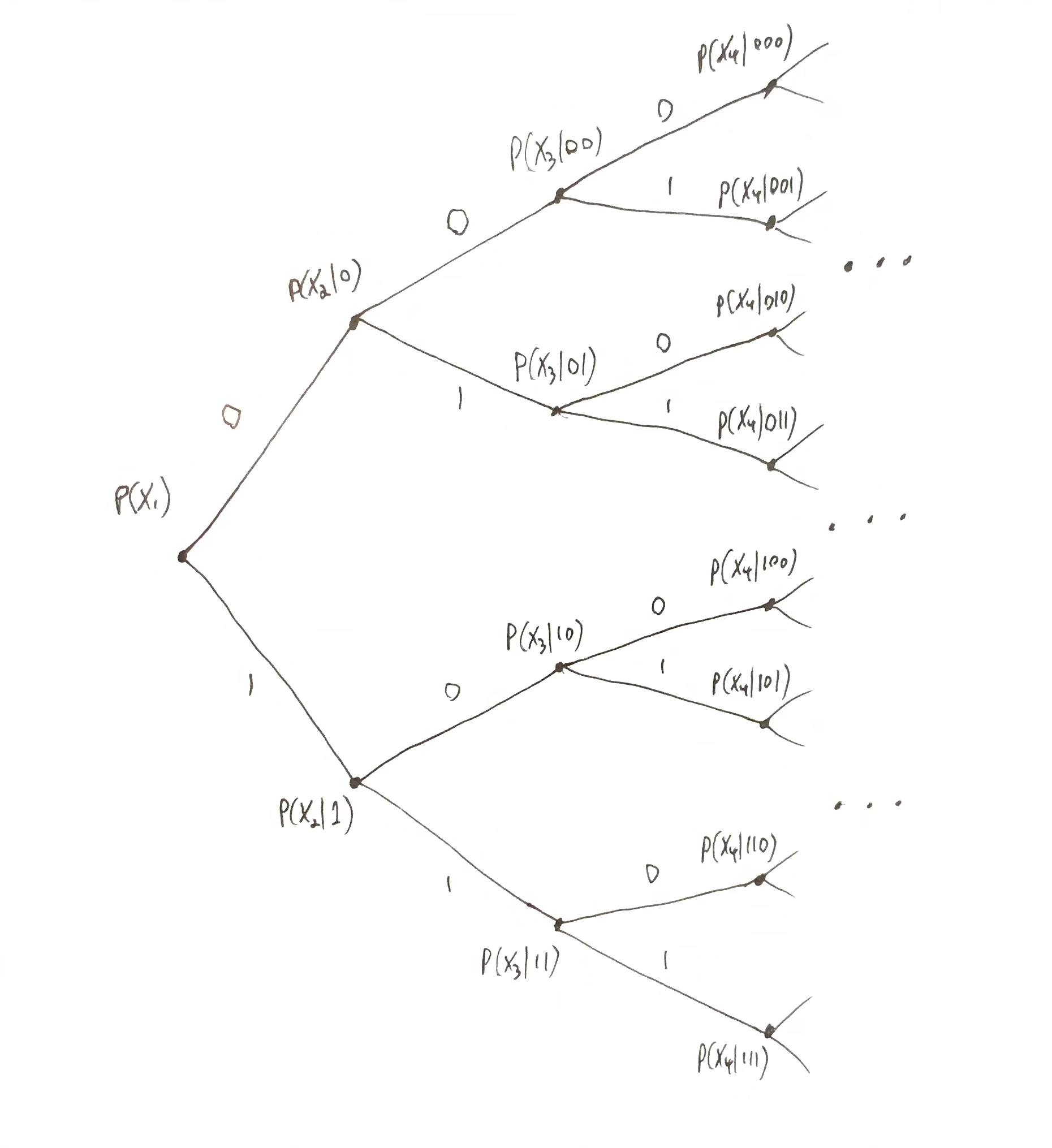
Each node in the tree is assigned a conditional probability distribution, i.e. for each node at position $x_{<n}$ (where $x_{<n} = (x_1, x_2,\dots,x_{n-1})$ encodes a path from the root), the probability $p(\chi \mid \dots)$ is specified for each $\chi\in\X$.

Each node’s distribution, $p(\chi \mid \dots)$, can be chosen independently from every other node (there are no constraints on these conditional distributions). Therefore, since the entire tree uniquely determines $p(x_{<n})$ (by walking down the edges of the tree corresponding to the observed data sequence $x_{<n}$ and multiplying the conditional probabilities at each node in the path, i.e. $p(x_i \mid x_{<i})$ at node $x_{<i}$), a Bayesian agent is free to choose any arbitrary conditional predictions it wants.

Clearly, if we are only concerned with data predictions of the form $p(\o_{n:m}\mid \o_{<n})$, then we do not actually need hypotheses at all. Providing a tree specifying the subjective conditional data probabilities is enough to perform Bayesian inference.

This reveals something peculiar about Bayesian inference: A Bayesian agent chooses its predictions for all eventualities beforehand, and never deviates for all time. Furthermore these predictions can be totally arbitrary. There does not appear to be any actual learning taking place, since the agent just follows a path down the tree as data comes in and provides predetermined prediction probabilities. In the Bayesian perspective, learning IS narrowing down a pre-defined possibility space with data. If decision making using Bayesian inference is rational, perhaps rationality amounts to consistency, i.e. never deviating from pre-chosen predictions.

One might argue that freely choosing a subjective data distribution without defining hypotheses is not Bayesian. My reply is that I’ve shifted what we are counting as hypothesis. In this perspective, a hypothesis is a single data sequence continuation. In this sense, all hypotheses are deterministic data sequences (though they may be algorithmically random), and the subjective data distribution is counting up the contributions of all these hypotheses to each finite length prediction. More on this in Bayesian information theory.

Removing probabilities

We can go a step further and ask, do we need probabilities at all?

Let’s imagine that the agent has the same predetermined tree as above, except each node is assigned a single prediction instead of a probability distribution over $\X$. Let $x\in\X^*$ and denote $\hat{\x}_x\in\X$ as the prediction given the sequence $x$ is observed. Choosing $\hat{\x}_x$ for each $x$ uniquely defines a tree, where $x = (x_1, x_2, \dots)$ encodes a path from the root to a node, and $\hat{\x}_x$ is the value assigned to that node.

Consider an example. Suppose $\X = \set{0,1}$ and that we have the following prediction tree:

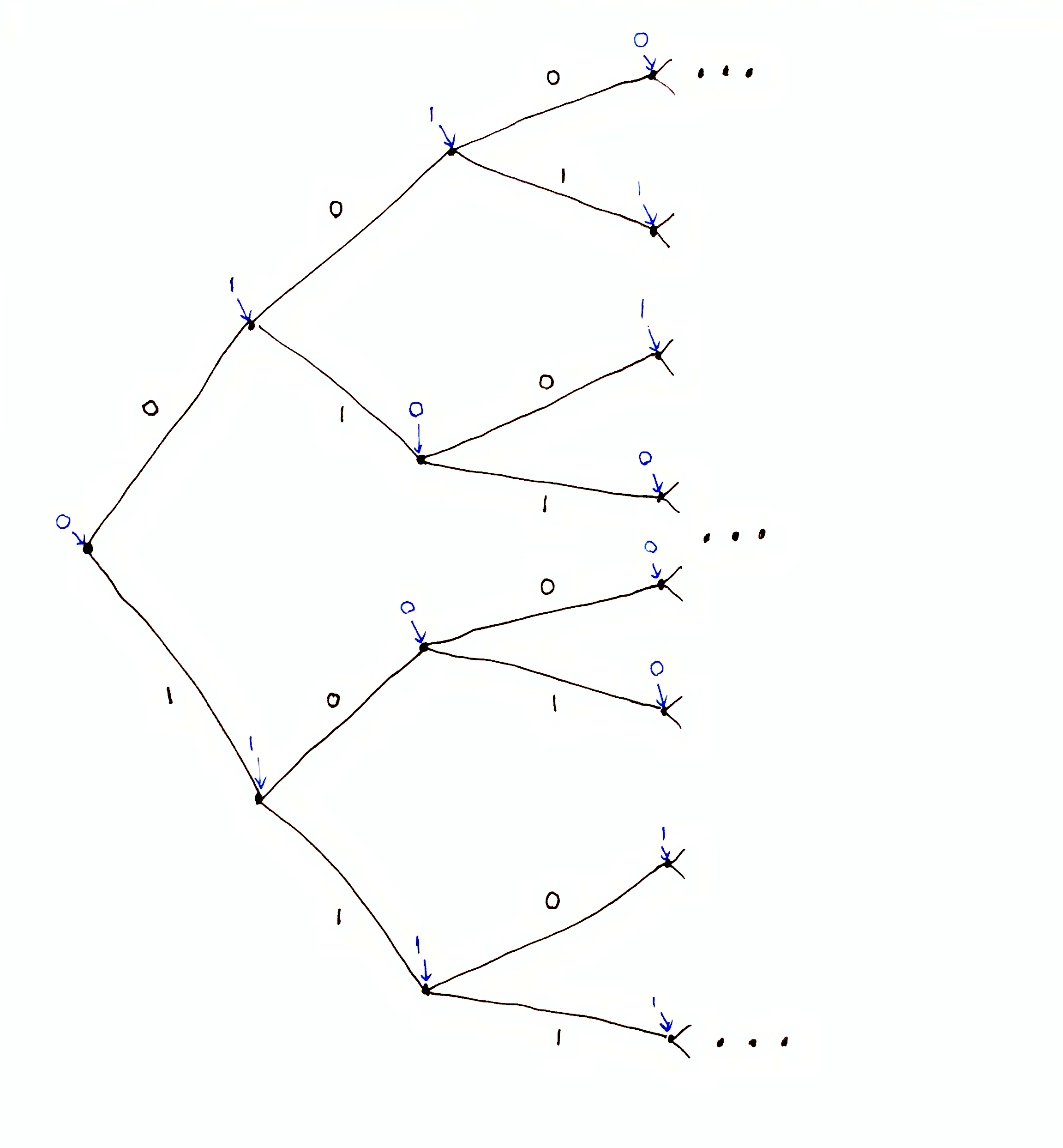
This tree has infinite depth.

In the figure, each node is assigned a prediction. Without any data, the agent predicts $0$. Given $0$ is observed, the agent predicts $1$. Given $01$ is observed, the agent predicts $0$. And so on.

Suppose we observe $010$, which falls in line with all of the agent’s predictions up to that point. The prediction given $010$ is $1$. Suppose we observe $0$ next (for a total observation of $0100$). Then the agent’s prediction of $1$ is wrong, but that is okay since the agent has sub-tree at $0100$ and can go on making predictions from there.

Is this setup technically Bayesian? We could convert this deterministic prediction tree to a subjective data distribution that assigns a probability 0 or 1 to all outcomes. So in this example, $p(x_1=0) = 1$ and $p(x_1=1)=0$, corresponding to a prediction of $0$ given nothing. $p(x_2=0\mid 0)=0$ and $p(x_2=1\mid 0)=1$, and $p(x_3=0\mid 01)=1$ and so on.

The problem is that $p$ defined in this way is degenerate. Suppose the agent wrongly predicts the continuation of $010$ to be $1$ when it is actually $0$. Then

$$
\begin{aligned}
p(0101) &= p(x_4=1\mid 010)p(x_3=0\mid 01)p(x_2=1\mid 0)p(x_1=0) \\ &= 1\cdot 1\cdot 1\cdot 1 = 1\,.
\end{aligned}$$

But $p(0100) = p(x_4=0 \mid 010)\dots = 0\cdot 1\cdot 1\cdot 1 = 0$. So from then on, the subjective probability of the data continuing $0100$ is 0, but the conditional probabilities may not be. If $p$ is defined as a measure on $\X^\infty$ instead of indirectly via the conditional probabilities specified in the tree, then $p$ cannot simultaneously have well-defined conditional probabilities and zero probability unconditionally (e.g. $p(x_5=0 \mid 0100) = 1$ while $p(01000) = 0$ and $p(0100) = 0$).

We might conclude that this kind of deterministic prediction tree does not formally conform to the definition of Bayesian inference I gave earlier. However, this tree is the limit of the probabilistic prediction tree above as each conditional probability $p(x_i \mid x_{<i})$ goes to 0 or 1. Just as the Dirac delta distribution is not technically a function, but can be defined as the limit of Gaussian functions as their variance goes to 0, we might be able to do the same with deterministic prediction trees.

Note that an agent that makes the same prediction no matter what is observed (a rigid agent) is technically Bayesian, with a subjective data distribution that puts all probability mass on the prediction sequence $\o\in\X^\infty$:

$$
p(x_{1:n}) = \begin{cases}1 & x_{1:n} = \o_{1:n} \\ 0 & x_{1:n} \neq \o_{1:n}\end{cases}
$$

Such an agent is not interesting, as it does not even behave as though it learns.

We shall see that an agent that does behave as though it learns (conditionally determines its predictions based on past history) need not provide Bayesian probabilities on its predictions for prediction uncertainty to naturally emerge.

Reconstructing Bayesian Inference

Non-Determinism

To add clarity to what I want to explain next, let’s represent the deterministic prediction tree above as a prediction function $f : \X^* \to \X$, so that $f(x) = \hat{\x}_x$ is the prediction given data sequence $x\in\X^*$. That is to say, $f(x)$ returns the value at node $x$ in the tree. We can think of $f$ as an assignment function of values to nodes.

Suppose we want to predict what will happen further out into the future. Specifically, suppose we observe $\o_{<n}\in\X^*$ and we want to predict the outcome $\o_m$ at time $m > n$. We don’t have access to the outcome $\o_n$ or anything after it. That is to say, the prediction tree gives the prediction $f(\o_{<n})$ for step $n$, but to predict step $m$ we need $\o_{<m} = \o_{<n}`\o_{n:m-1}$.

You might say that the solution is to fill in our missing data with predictions, i.e. choose $\hat{\o}_n=f(\o_{<n})$ as the outcome for step $n$, and $\hat{\o}_{n+1} = f(\o_{<n}`\hat{\o}_n)$ as the outcome for step $n+1$, etc., so that our prediction at step $m$ is $\hat{\o}_m=f(\o_{<n}`\hat{\o}_{n:m-1})$. However, I’d argue that this is not actually the agent’s prediction as defined by the prediction tree. If the agent instead observed $\o_{n:m-1} \neq \hat{\o}_{n:m-1}$, the agent might predict something different from $\hat{\o}_m$. We could define $\hat{\o}_m$ as the agent’s prediction of step $m$ given $\o_{<n}$. By doing so, we’d be assigning infinite sequences to each node $x$ in the prediction tree, rather than single outcomes, so that we may query the prediction of arbitrarily many timesteps given ONLY data $x$. We can represent this prediction tree by the function $g:\X^*\to\X^\infty$, which returns an infinite sequence in $\X^\infty$ instead of a single element of $\X$, such that $[g(x_{<n})]_{<n} = x_{<n}$ and $[g(x_{<n})]_n$ is the next-step prediction for $x_{<n}$. The sequence $[g(x_{<n})]_{\geq n}$ is the multi-step prediction for $x_{<n}$. Now it is clear that $[g(\o_{<m})]_m$ and $[g(\o_{<n})]_m$ are potentially different predictions, and we need to distinguish between them.

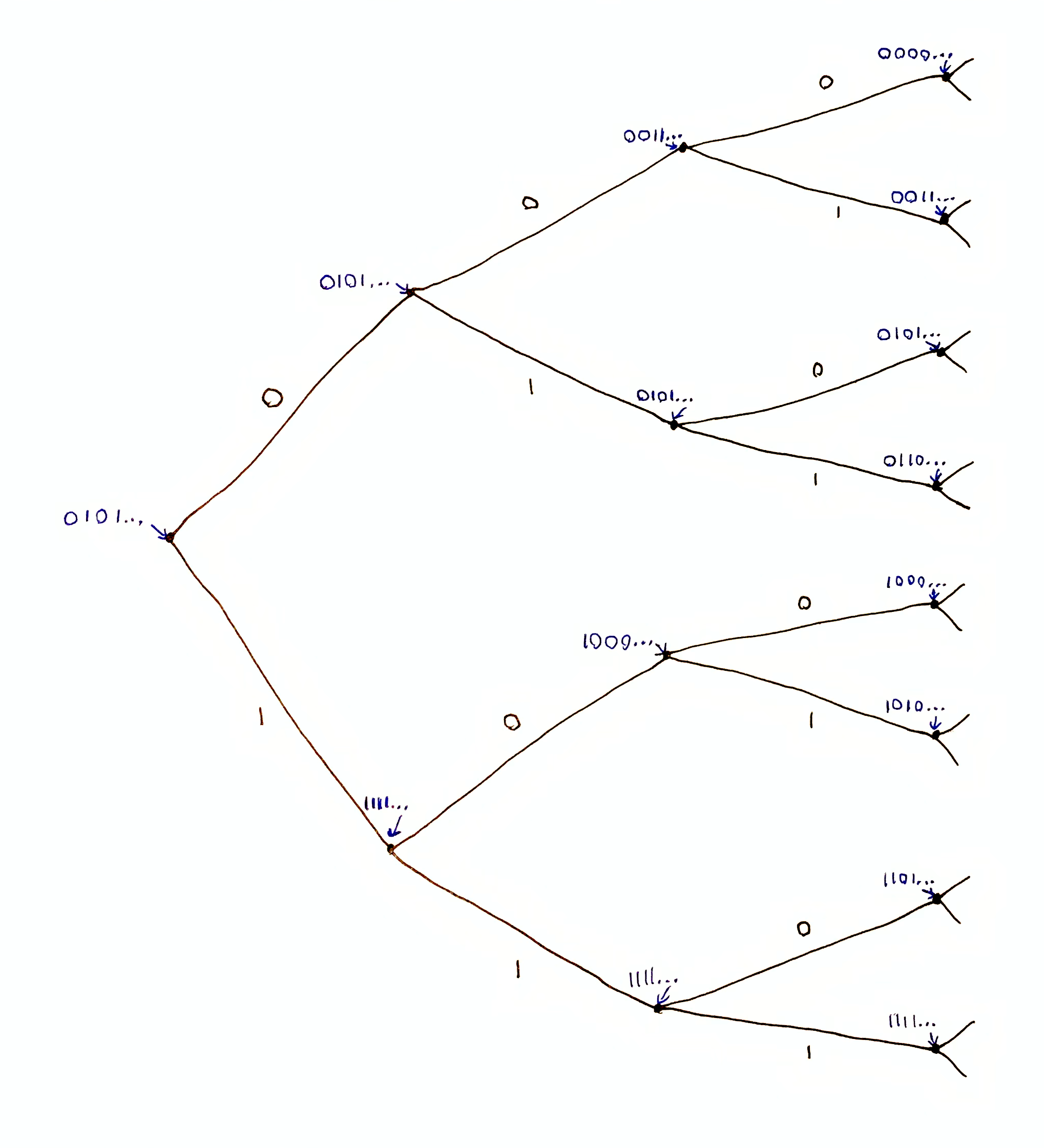
The tree encoded by $g$, where each node is assigned an infinite sequence that begins with the location of the node in the tree. In this example, each sequence is the argmax prediction starting at that node, i.e. assuming every next-step prediction is correct.

In general, if we ask an agent for some prediction of any time-step, the agent can produce some sort of answer. However, if we wanted to know what answer the agent would produce if all requisite data was available (call this the agent’s best prediction), that may not be determinable with the data currently available. We are uncertain about what the agent’s best prediction will be (given all requisite data). A truthful agent would be just as uncertain as we are about its own future predictions.

Let $\mc{F}_m(\o_{<n}) = \set{f(\o_{<n}`\tilde{\o}_{n:m-1}) \mid \tilde{\o}_{n:m-1}\in\X^{m-n+1}}$ be the set of all predictions the agent could make about step $m$ given data $\o_{<n}$. If this set contains more than one element, then the agent’s prediction at $m$ is not uniquely determined by $\o_{<n}$, i.e. non-deterministic.

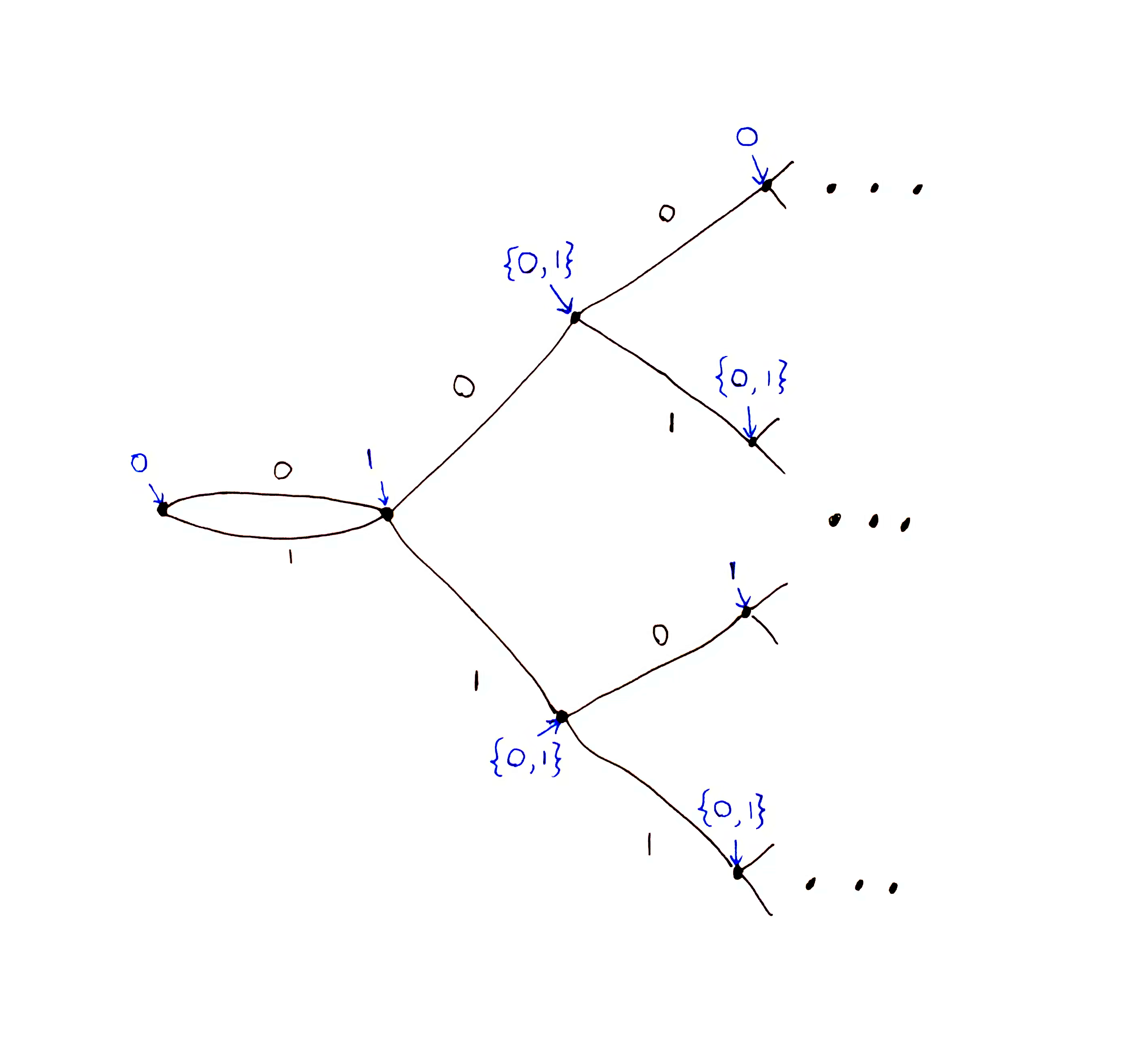
This is the non-deterministic prediction encoded by $\mc{F}_2 : \X^* \to \X$, where the untransformed tree encoded by $f:\X^*\to\X$ is our prediction tree example from above. $\mc{F}_2$ is obtained by superimposing the two sub-trees of $f$ at depth 1, i.e. directly under the root node.

This understanding of the word “non-deterministic” is standard in computer science, exemplified by the non-deterministic Turing machine, which defines a set of possible state transitions and tape operations given any state (of both the tape and automata), rather than single one determined uniquely by each state. In general, something is regarded as non-deterministic if it can take on more than one possible value, i.e. it is not determined.

I distinguish non-determinism from randomness, the latter of which can be defined as maximal incompressibility (called algorithmic randomness). Often these two concepts are conflated. Probability distributions can represent both non-determinism (by quantifying relative amounts of possibilities) or degrees of randomness (via Martin-Lof randomness). The key insight is that probability need not represent both at the same time. If Bayesian probability is generally understood as quantifying prediction non-determinism, then we can view the Bayesian-frequentist distinction as stemming from this conceptual decoupling of non-determinism from randomness.

I make the same connection between Bayesian uncertainty and non-determinism in Classical vs Bayesian Reasoning.

The General Case

We can go a step further. Why are we assuming that a prediction of step $n$ can be made given $\o_{<n}$? Plenty of pertinent information may not be available in the data at all (or the agent does not know how to extract such information from the data, e.g. encrypted information). An honest agent would account for every input needed to make a certain prediction, even inputs that are not available in $\o_{<n}$.

In general, we are left with a non-deterministic next-step prediction tree represented by $f : \Z \times \X^* \to \X$ where $\Z$ is an auxiliary input space (input in addition to the observed data stream), which is usually some latent space (set of possible data or world-states not observed). Each node $x$ in the prediction tree is assigned the prediction set $f(\Z, x) = \set{f(z,x) \mid z\in\Z}$. If the prediction set for $x$ is singleton (contains one element), then that prediction is deterministic. $f$ represents a prediction tree where each node is assigned a set of next-step predictions instead of just one.

The Return Of Probability

In Classical vs Bayesian Reasoning, I introduced the Bayesian axiom - an informal axiom of epistemology - which states that the relative fraction of model (in our case $f$) inputs which produce each output can be regarded as knowledge. In this case, if the agent’s prediction $f(\Z, \o_{<n})$ is not uniquely determined, we might want to proceed with our decision making anyway. Supposing we have some normalized measure $\mu$ on $\Z$ (ideally the uniform measure if there is one), then the relative fraction of $\Z$ that produces each prediction $\chi\in\X$ is

$$p(\chi \mid x) = \mu\set{f(z,x) \mid z\in\Z \and f(z,x) = \chi}\,.$$

Though the agent’s prediction is not uniquely determined, we’ve quantified the relative number of possible auxiliary inputs to $f$ that give each prediction. These quantities can be used for decision making (e.g. most likely outcome or expected return).

We have recovered the probabilistic prediction tree paradigm from earlier without presupposing that predictions should be probabilistic. Though not defined to be probabilistic, an agent’s prediction function that requires inputs which are not on hand naturally results in non-determinism. Quantifying that non-determinism using relative sizes of possibility sets naturally results in probabilities.

With this perspective in mind, we could interpret any explicitly defined subjective data distribution to be implying the existence of a deterministic prediction function. Bayesian probabilities represent the number of inputs to this prediction function that produce the corresponding outputs. Given $p$, a canonical deterministic prediction function $f$ is the decoder for a compressed representation of the data, with a uniform distribution on the compression.

To be more specific, let $p$ be a probability measure on $\X^\infty$. Let $f : \Z^\infty \to \X^\infty$ be an arithmetic decoder using $p$, i.e. $f$ takes as input an infinite compressed sequence $z_{1:\infty}\in\Z^\infty$ and outputs the decompressed sequence $x_{1:\infty}\in\X^\infty$. For finite inputs and outputs, use the cylinder set $f(\Gamma_{z_{1:n}})$. Putting a uniform probability measure on $\Z^\infty$ results in measure $p$ on $\X^\infty$. Now we can draw a connection between probability in three different contexts:

• Shannon Information
  • If $x_{1:\infty}$ is sampled randomly from $p$, then $z_{1:\infty}$ s.t. $f(z_{1:\infty}) = x_{1:\infty}$ achieves the optimal compression of $x_{1:\infty}$ according to Shannon. That is to say, $\abs{z_{1:n}} = n \approx -\lg p(f(\Gamma_{z_{1:n}}))$, and these quantities converge as $n\to\infty$.
• Algorithmic Randomness
  • If input $z_{1:\infty}$ is algorithmically random, then output $f(z_{1:\infty})$ is $p$-random (or $p$-typical, see wiki). $z_{1:\infty}$ is a shortest algorithmic compression of $f(z_{1:\infty})$.
• Non-determinism
  • Our prediction of $x_n$ given $x_{<n}$ depends on the compressed representation of $x_{1:n}$, an input $z_{1:k}$ to $f$ s.t. $f(\Gamma_{z_{1:k}}) = \Gamma_{x_{1:n}}$. Our non-deterministic prediction of $x_{n}$ given $x_{<n}$ is the set $f^{-1}(\Gamma_{x_{1:n}})$, which is all compressions compatible with $x_{1:n}$. This is quantified with the probability $p(x_n \mid x_{<n}) = \lambda(f^{-1}(\Gamma_{x_{1:n}})) / \lambda(f^{-1}(\Gamma_{x_{<n}}))$ where $\lambda$ is the uniform probability measure on $\Z^\infty$.

Use Cases

This section runs through a few canonical examples of Bayesian inference which can be used as intuition pumps while reading the previous sections.

Inferring bias on a coin

Let $\X = \set{0,1}$ be the outcome of a coin toss, and $\o \in \X^\infty$ be an infinite sequence of coin toss outcomes.

Let $\mc{B}_\t$ be the Bernoulli distribution on $\X$ with parameter $\t\in[0,1]$ which is the probability of $1$, so $\mc{B}_\t(1) = \t$ and $\mc{B}_\t(0) = 1-\t$.

The hypothesis $\mu_\t$ is the product of Bernoulli distributions:

$$
\mu_\t(x_{1:n}) = \prod_{i=1}^n\mc{B}_\t(x_i) = \t^{\sum_i x_i}(1-\t)^{n-\sum_i x_i}\,.
$$

The hypothesis set is $\H = \set{\mu_\t}_{\t\in[0,1]}$. These hypotheses are i.i.d. w.r.t. sequence position, i.e. $\mu_\t(x_n \mid x_{<n}) = \mu_\t(x_n)$.

Subjective data probability:
$$
p(x_{1:n}) = \int_0^1 p(\t)\mu_\t(x_{1:n}) d\t = \int_0^1 p(\t)\t^{\sum_i x_i}(1-\t)^{n-\sum_i x_i} d\t
$$

Data posterior:
$$
p(x_n \mid x_{<n}) = \int_0^1 p(\t\mid x_{<n})\mu_\t(x_n \mid x_{<n})d\t = \int_0^1 p(\t\mid x_{<n})\mc{B}_\t(x_n)d\t
$$

Hypothesis posterior:
$$
p(\t\mid x_{1:n}) = p(\t)\frac{\mu_\t(x_{1:n})}{p(x_{1:n})}
$$

Note that the hypotheses are i.i.d. w.r.t. data position but the subjective data distribution $p$ is not. That is to say, $\mu_\t(x_n \mid x_{<n}) = \mu_\t(x_n)$ but $p(x_n \mid x_{<n}) \neq p(x_n)$.

Solomonoff Induction

Let’s continue the coin tossing example, but instead of coin tossing, suppose any arbitrary process that produces a binary data stream. That is to say, we are allowing dependencies between bits in the data sequence.

Bernoulli hypotheses are blind to patterns in the ordering of bits in the data sequence because $\mu_\t(x_{1:n}) = \mu_\t(\mathrm{permute}(x_{1:n}))$ where $\mathrm{permute}(x_{1:n})$ is any permutation (re-ordering) of $x_{1:n}$. For example, we observe a very long sequence of alternating $0$s and $1$s, i.e. $0101010101\dots$, then the Bernoulli hypothesis where $\t=1/2$ will get large posterior weight. This is the hypothesis that the data is totally random (maximum entropy). Clearly, the data is highly patterned and predictable.

What hypotheses should we add to $\H$? Is it possible to have a hypothesis for every possible data pattern? Ray Solomonoff’s answer is yes, and this is achieved by the hypothesis set containing all semicomputable semimeasures on $\X^\infty$.

A probability measure $\mu$ on $\X^\infty$ is computable if there exists a program (Turing machine) which outputs the probability $\mu(x_{1:n})$ of any input, $x_{1:n} \in \X^n$ (for any $n\in\mb{N}$), to the requested precision, $\e > 0$, in finite time and then halts. Alternatively, a probability measure is computable if there exists a program that outputs each possible outcome $x_{1:n} \in \X^n$ (for any $n\in\mb{N}$) with probability $\mu(x_{1:n})$, given a stream of uniformly random input bits (i.i.d. Bernoulli(1/2) data).

A probability measure $\mu$ on $\X^\infty$ is semicomputable if there exists a program (Turing machine) which outputs an infinite monotonic (increasing or decreasing) sequence of rational numbers $(\hat{q}_i)_{i\in\mb{N}}$ s.t. $\hat{q}_i$ converges to $\mu(x_{1:n})$ as $i\to\infty$, for any $x_{1:n} \in \X^n$ (for any $n\in\mb{N}$). All computable measures are semicomputable. A semicomputable measure is not computable if the error $\e_i = \abs{\hat{q}_i - \mu(x_{1:n})}$ at position $i$ in the output sequence cannot be computably determined. If this error could be determined, this program can be converted into the one above that approximates $\mu(x_{1:n})$ to the desired error in finite time. In other words, a semicomputable measure can be approximated to arbitrary accuracy, but you may not be able to determine how close any given approximation is, whereas a computable measure can be arbitrarily approximated with known error.

A semimeasure $\mu$ on $\X^\infty$ is like the measure we defined earlier in #Defining A Hypothesis except for one difference: Rather than strict equality we have

$$
\mu(x_{<n}) \geq \int_\X \mu(x_{<n}`\chi)d\chi\,.
$$

For $\X = \set{0,1}$, this property becomes

• Measure: $\mu(x_{<n}) = \mu(x_{<n}`0) + \mu(x_{<n}`1)$
• Semimeasure: $\mu(x_{<n}) \geq \mu(x_{<n}`0) + \mu(x_{<n}`1)$

Note that $0 \leq \mu(x_{<n}) \leq 1$ still holds. We just allow probabilities to sum to less than 1.

The set of all computable measures is conceptually nicer to think about than (and is a subset of) the set of all semicomputable semimeasures, but is not practically useful because it cannot be enumerated by a program, i.e. is computably enumerable (c.e.). To enumerate this set, you’d have to determine which programs halt after emitting their approximation of $\mu(x_{1:n})$.

The set of all semicomputable semimeasures can be enumerated by a program, by enumerating all programs in lexicographic order, running them all simultaneously (called dovetailing, see also c.e. set), and continually filtering out the programs whose output does not compute a valid semimeasure. The virtue of using semimeasures rather than measures is that we don’t need to wait for the programs being enumerated to halt. If one is found to violate the semimeasure property (probabilities sum to greater than 1) it is filtered out. Otherwise it remains and we don’t have to check that the probabilities it assigns to various outcomes sum to exactly 1 (which would require waiting for it to halt).

Let hypothesis set $\H$ be the set of all semicomputable semimeasures. Then the subjective data distribution is also a semicomputable semimeasure:

$$
p(x_{1:n}) = \sum_{\mu\in\H} p(\mu)\mu(x_{1:n})\,.
$$

Solomonoff makes a prescription on what prior to use:

$$
p(\mu) = 2^{-K(\mu)}
$$

where $K(\mu)$ is the prefix-free Kolmogorov complexity of hypothesis $\mu\in\H$. This prior weights hypotheses inversely by complexity - a sort of Occam’s razor.

Machine Learning

We have a family of functions $\set{h_\t}_{\t\in\T}$ with signature $h_\t : \X \to \Phi$ (for example, $h_\t$ could be a neural network), where $\Phi$ is the parameter space for a probability distribution $\P$ on the space $\Y$. That is to say, $\P(y \mid h_\t(x))$ is the probability of $y\in\Y$ given $x\in\X$ according to the model $h_\t(x)$. We call $\X$ the input space, and $\Y$ the target (output) space.

We observe a data sequence $x_1y_1x_2y_2x_3y_3\dots x_n$ ending in $x_n$. Let $D = x_1y_1x_2y_2x_3y_3\dots x_{n-1}y_{n-1}$ be the training data. $x_n$ is called the test input. The goal is to predict the next element in the sequence, $y_n$.

We can take a Bayesian approach by defining the following hypothesis space:

$$
\H = \set{\mu_\t \mid \t\in\T}\,,
$$

where $\mu_\t$ is a probability measure on $\X\times\Y\times\X\times\Y\dots = (\X\times\Y)^\infty$ s.t. for all $\o\in(\X\times\Y)^\infty$ and for all $(x_i,y_i)\in\o$,

$$
\mu_\t(y_i \mid x_i) = \P(y_i \mid h_\t(x_i))\,.
$$

$\mu_\t$ is i.i.d. w.r.t. sequence position, i.e. $\mu_\t(y_i \mid x_i) = \mu_\t(y_i \mid x_1y_1\dots x_i)$. That is to say, all of our hypotheses assume the data is drawn i.i.d. (and so the data sequence $D$ becomes a dataset, in the sense that it is unordered). If we are doing supervised learning, then the marginal probabilities $\mu_\t(x_i)$ should all be uniform (the hypothesis is indifferent to which input $x\in\X$ comes next in the sequence). On the other hand, if we are doing unsupervised or semi-supervised learning, then $\mu_\t(x_i)$ should also depend on the model output $h_\t(x_i)$.

Finally, put a prior $p$ on the parameter space $\T$. Then the subjective probability of the test output $y_n$ given test input $x_n$ is the data posterior of $y_n$ given the data sequence $D`x_n = x_1y_1x_2y_2x_3y_3\dots x_n$:

$$
\begin{aligned}
p(y_n \mid D`x_ny_n) &= \int_\T p(\t\mid D`x_n)\mu_\t(y_n \mid D`x_n)d\t \\
&= \int_\T p(\t\mid D`x_n)\mu_\t(y_n \mid x_n)d\t
\end{aligned}
$$

where the parameter posterior is

$$
\begin{aligned}
p(\t\mid D`x_n) &= p(\t)\frac{\mu_\t(D`x_n)}{p(D`x_n)}
\end{aligned}
$$

In the supervised case $\mu_\t(x_1) = \mu_\t(x_2) = \dots = \mu_\t(x_n) = \gamma$, and so $\mu_\t(D`x_n) = \gamma\mu_\t(D)$. Likewise, $p(D`x_n) = \int_\T p(\t)\mu_\t(D`x_n) d\t = \gamma\int_\T p(\t)\mu_\t(D) d\t$, and so the fraction $\mu_\t(D`x_n)/p(D`x_n)$ simplifies to $\mu_\t(D)/p(D)$. Then the parameter posterior reduces to the classic form: $p(\t\mid D`x_n) = p(\t\mid D) = p(\t)p(D\mid \t)/p(D)$. where $p(D\mid \t) = \mu_\t(D)$.