
[This is an article, which is something I’ve optimized for readability and transmission of ideas, opposed to notes that are the seed of an idea and something I’ve written quickly.]
My goal is to identify the core conceptual difference between someone who accepts “Bayesian reasoning” as a valid way to obtain knowledge about the world, vs someone who does not accept Bayesian reasoning, but does accept “classical reasoning”. By classical reasoning, I am referring to the various forms of logic that have been developed, starting with Aristotelian logic, through propositional logic like that of Frege, and culminating in formal mathematics (e.g. higher order type theory). In such logics, the goal is to uniquely determine the truth values of things (such as theorems and propositions) from givens.
My thesis is that the difference between Bayesian and classical reasoners comes down to how they deal with undetermined objects (e.g. if you cannot determine the truth value of something from your givens). The classical reasoner will shrug their shoulders and say “the answer cannot be determined, collect more givens or modify your definitions”. The Bayesian reasoner will consider all the variables with unknown values that, combined with the givens, would fully determine the target propositions. Then the Bayesian reasoner will consider the set of all possible values of those unknown variables and subset of possibilities that make the target propositions true. The Bayesian reasoner measures the sizes of both sets and considers the fraction of unknown values that make the target propositions true to be epistemologically salient. This last bit is the key distinction between the classical and Bayesian reasoners. This is the mechanism by which the Bayesian reasoner continues on without uniquely determined truth values, while the classical reasoner does not.
This difference extends beyond epistemology into the realm of machine learning. Classical epistemology is interested in truth (i.e. uniquely determined quantities), whereas Bayesian epistemology is interested in degrees of certainty. In machine learning, the givens and unknowns in question are not boolean valued, but have arbitrary data types (e.g. vectors of reals). The classical learner is interested in what numbers can be uniquely determined from data, and the Bayesian learner is interested in proportions of possibilities that result in each number.
This philosophical difference leads to a practical methodological difference. A classical reasoner/learner will define universes such that unknowns can be uniquely determined. Otherwise, the definitions are not useful. A Bayesian reasoner/learner will define universes such that calculating posterior probabilities are tractable. Otherwise, the definitions are not useful.
A note on the definition of model. In mathematics, a model is an instantiation of an unspecified object which satisfies given axioms. In machine learning, a model refers to a family of instantiations of free parameters, i.e. a model is the set of definitions which invoke free variables that are to be determined.
$$
\newcommand{\0}{\mathrm{false}}
\newcommand{\1}{\mathrm{true}}
\newcommand{\mb}{\mathbb}
\newcommand{\mc}{\mathcal}
\newcommand{\and}{\wedge}
\newcommand{\or}{\vee}
\newcommand{\a}{\alpha}
\newcommand{\t}{\theta}
\newcommand{\T}{\Theta}
\newcommand{\o}{\omega}
\newcommand{\O}{\Omega}
\newcommand{\x}{\xi}
\newcommand{\fa}{\forall}
\newcommand{\ex}{\exists}
\newcommand{\X}{\mc{X}}
\newcommand{\Y}{\mc{Y}}
\newcommand{\Z}{\mc{Z}}
\newcommand{\P}{\Psi}
\newcommand{\y}{\psi}
\newcommand{\p}{\phi}
\newcommand{\B}{\mb{B}}
\newcommand{\m}{\times}
\newcommand{\E}{\mc{E}}
\newcommand{\e}{\varepsilon}
\newcommand{\set}[1]{\left\{#1\right\}}
\newcommand{\abs}[1]{\left\lvert#1\right\rvert}
\newcommand{\inv}[1]{{#1}^{-1}}
\newcommand{\Iff}{\Leftrightarrow}
$$
Propositional logic
The math perspective
I will be using the example in Russell and Norvig’s Artificial Intelligence: A Modern Approach (3rd edition), chapter 7.
We are introduced to “wumpus world”, a grid world containing an enemy called the wumpus, death pits, and gold.
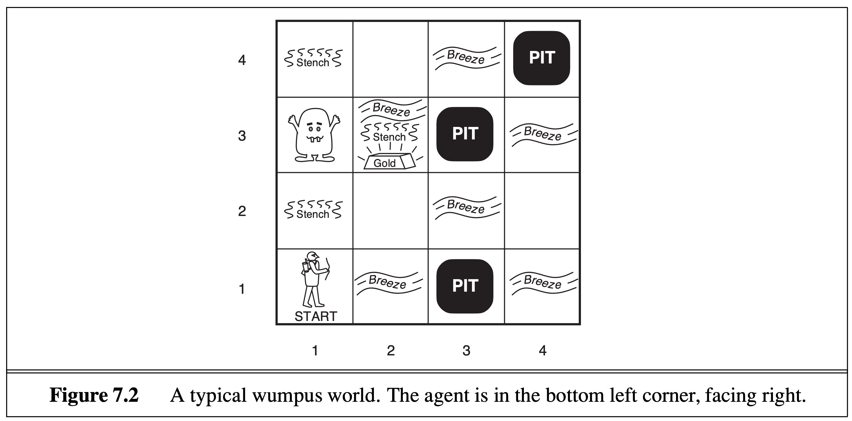
The relevant rules are:
- the agent starts in the bottom left corner
- the agent can only see what is contained in the cell it currently occupies
- the agent will detect a “breeze” if it’s cell is adjacent to a pit
- if the agent moves into a pit, it dies
- the goal is to get to the gold
Suppose the agent moves right:
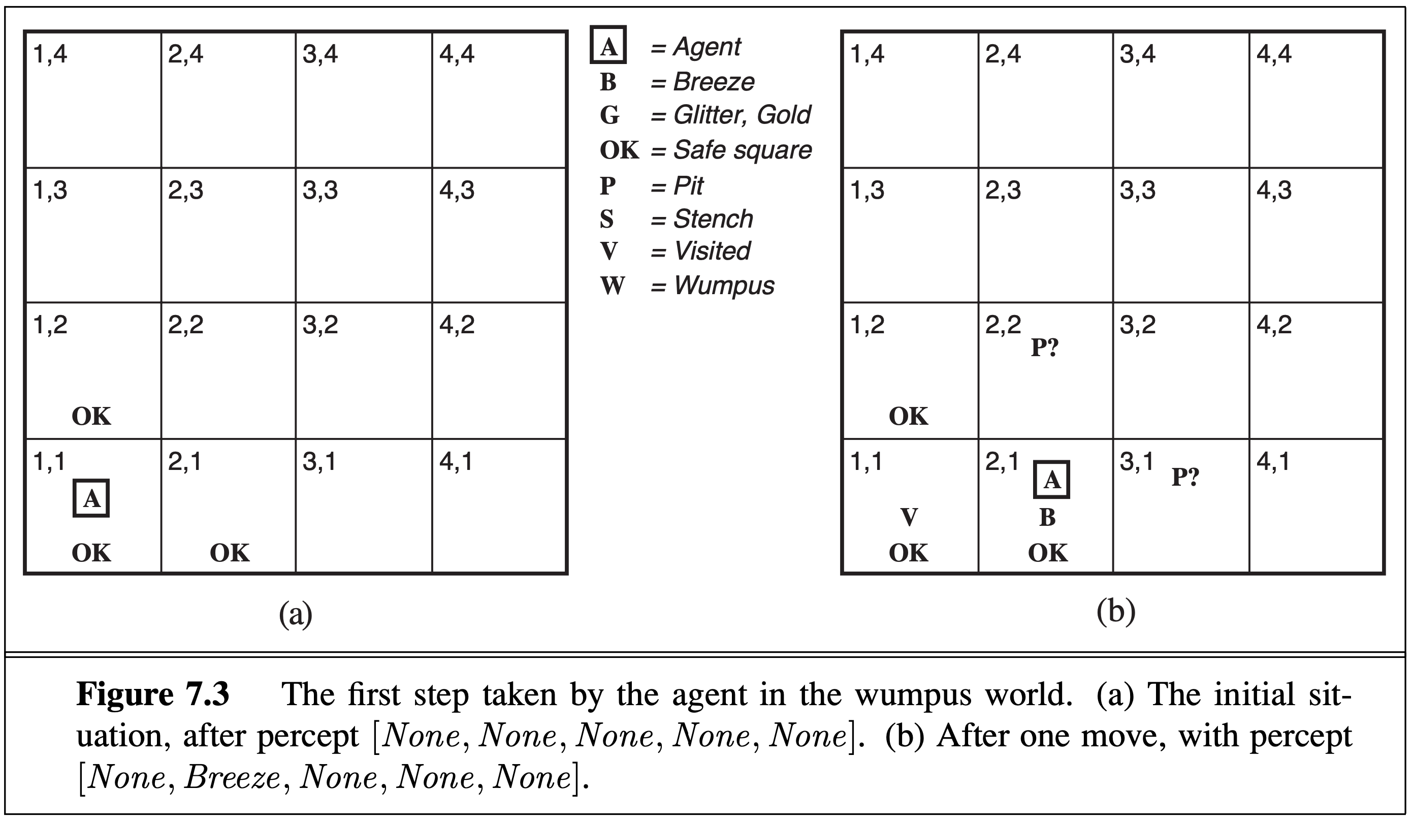
No breeze is detected in the starting cell [1,1], so the agent knows there is no pit up or to the right. In cell [2,1], there is a breeze, so the agent knows there is a pit above or to the right (or both).
Each case can be defined by the following propositions: $P_{x,y}$ is instantiated as a different variable for each coordinate, i.e. $P_{1,1}, P_{1,2}, P_{2,1},\ldots$ are all different variables.
We define the following boolean variables:
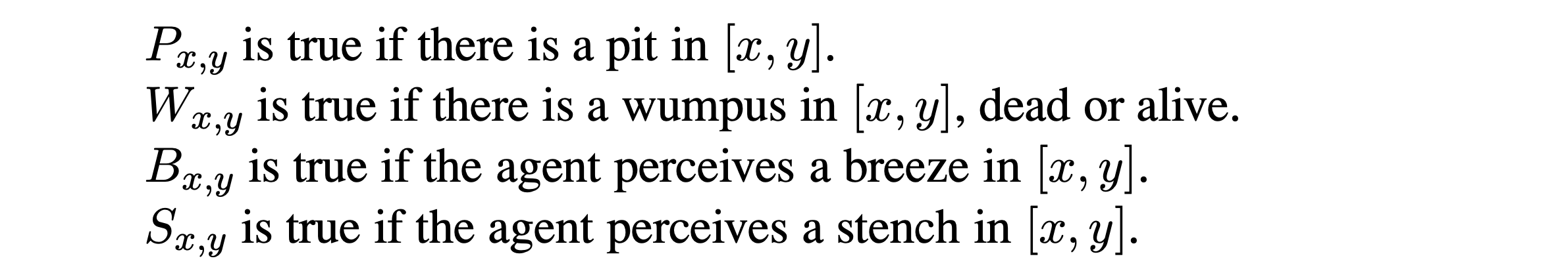
A model (in the math sense) is an instantiation of these variables (in contrast to the machine learning sense where a model is the entire definition of the game and all the variables). There are 4 variables for each coordinate, and 16*4 = 64 variables in total. Thus a model can be viewed as a length 64 boolean vector. Suppose $m$ is such a vector. Then if $\a_1$ is true for $m$, we say that $m$ is a model of $\a_1$.
Let $M(\a)$ be the set of all models (i.e. length 64 boolean vectors) satisfying some arbitrary sentence $\a$. Let $\beta$ be another sentence. We say that $\a$ entails $\beta$, notated $\a \models \beta$, iff $M(\a) \subseteq M(\beta)$.
Diagrammatically, we can depict the sets $M(\a_1)$ and $M(\a_2)$ (referring to the sentences above), as well as our knowledge base (KB) (i.e. what is given):
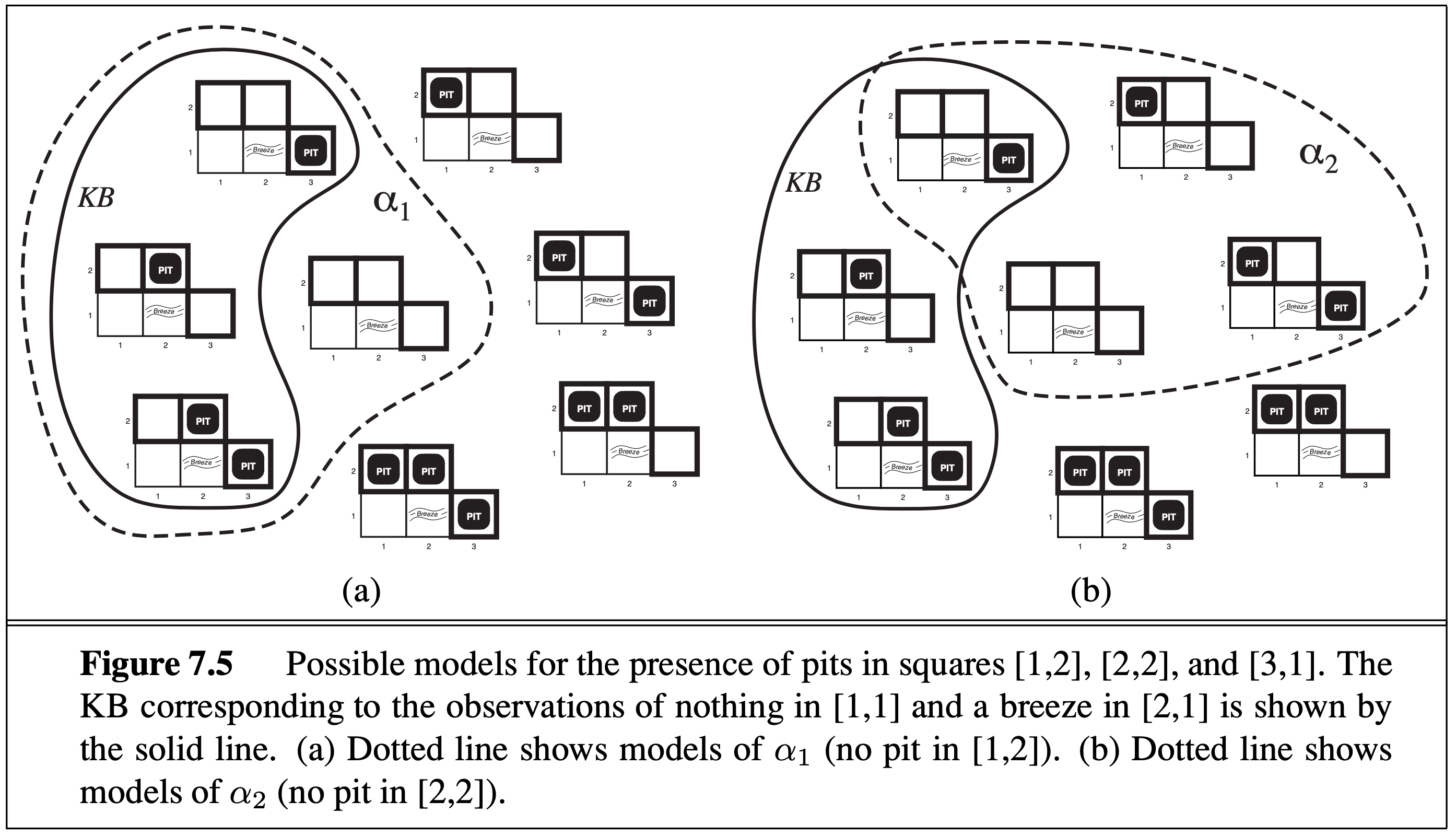
In our wumpus world, the “sentences” above can be formally states as propositions, along with the rules for the game:
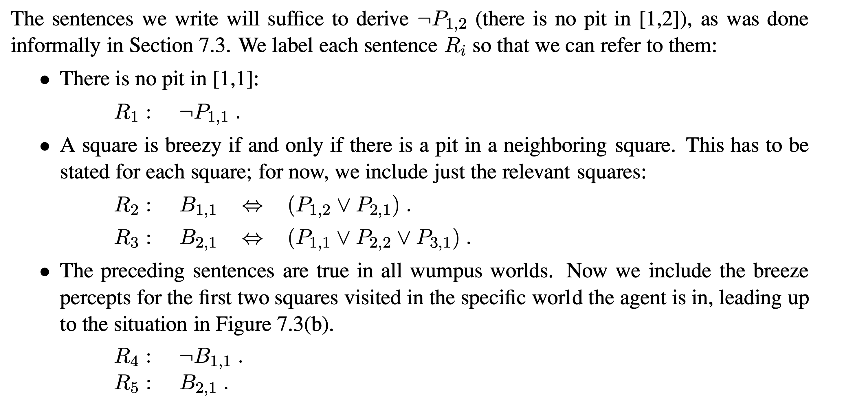
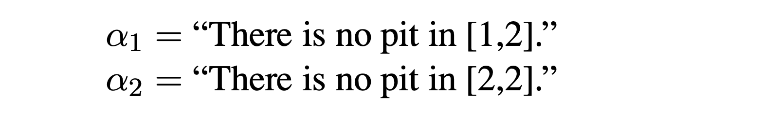
We can prove simple things like “there is no pit in [1,2]” using the rules of logical inference. The following propositions are true in all models where $R_1,\ldots,R_5$ are true:
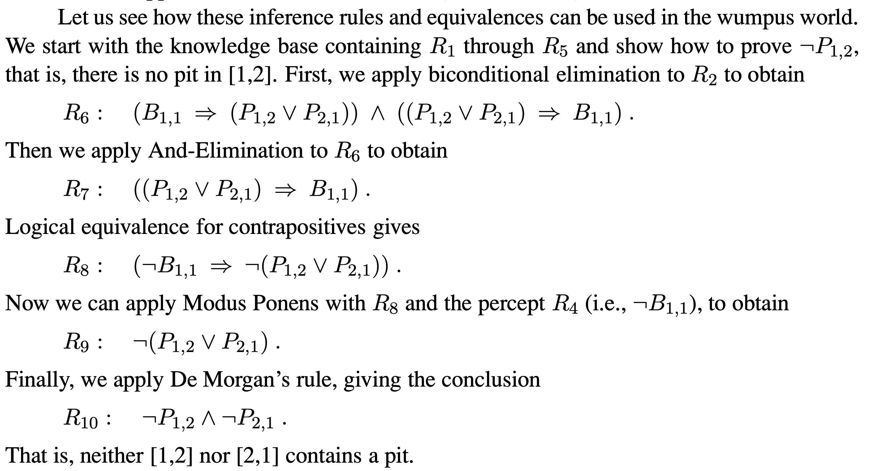
Each $R_i$ is entailed by the proceeding $R_j$ for $j < i$. A sequence of such propositions resulting in a desired proposition is a proof. From $R_{10}$, we can conclude $\neg P_{1,2}$. This sequence of propositions is a proof of $\a_1$ = “there is no pit in [1,2]”.
We can also verify the statement $\a_1$ is true with brute force instead of logical inference: by enumerating all models ($2^{64}$ of them), selecting the models which satisfy $R_1,\ldots,R_5$ (i.e. $M(R_1\and\ldots\and R_5)$), and then checking if $\neg P_{1,2}$ is true in all of them.
Notice that we cannot prove $P_{2,2}$ or its negation $\neg P_{2,2}$ given $R_1,\ldots,R_5$. That is because some models of $R_1\and\ldots\and R_5$ are consistent with $P_{2,2}$ while others are consistent with $\neg P_{2,2}$. That is to say, the truth value of variable $P_{2,2}$ is not uniquely determined by the givens $R_1,\ldots,R_5$. Speaking informally, we do not have enough information to know whether there is a pit at [2,2]. Therefore a rational agent would not make decisions based on $P_{2,2}$ being true or false. This is a core tenet of classical logic, whereas we shall see later, a Bayesian reasoner might be able to do more with the same information.
The machine learning perspective
In machine learning, a model is a function $f : \O \to \X$, where $\O$ is called the state set, and $\X$ is called the observation set. This is different from the math notion of a model we saw above.
Typically $\O$ and $\X$ are each the Cartesian products of other primitive types (which are sets, e.g. the reals, the integers, the booleans, etc.). Thus elements of $\O$ and $\X$ are typically tuples. Each element of the tuple is called a dimension. Generally, $\O$ and $\X$ are high-dimensional (elements of $\O$ and $\X$ are very long tuples, possibly infinite).
An element $\o \in \O$ is called a state, and is considered to be a possible state of the world, where the world is the model. Often, $\O = \T\m\E$, where $\T$ is called the parameter set, and $\E$ is the noise set (both sets are themselves multi-dimensional). In the typical ML formulation, $\t\in\T$ is explicitly represented but $\e\in\E$ is not, because $\t$ is what is being “solved for” while $\e$ represents random inputs. In my formulation, I combine both into a single state $\o = (\t,\e)$. If $\o$ is some tuple, then a subtuple of $\o$ is called a substate, so $\t$ and $\e$ are substates of $\o = (\t, \e)$.
An element $x \in \X$ is called an observation. Usually we are only given a partial observation. If $\X = T_1 \m T_2 \m T_3 \m \dots$ for primitive types $T_1, T_2, T_3, \ldots$, then a full observation is $x = (t_1, t_2, t_3, \ldots) \in \X$. A partial observation is a subset of elements in the tuple $x$. We denote partial observations with subscripts: $x_{1,5,10}$ is the tuple $(t_1, t_5, t_{10})$. We can also take slices: $x_{a:b} = (t_a, t_{a+1}, \ldots, t_{b-1}, t_b)$ is the slice from index $a$ to $b$. The shorthand $x_{>a}$ is the tuple of all indices larger than $a$, and $x_{<a}$ is the tuple of all indices less than $a$. It is sometimes convenient to think of a partial observation $x_I$ (for index tuple $I$) as a subset of $\X$, i.e. the set of all $x\in\X$ satisfying the partial observation. For example, $x_{1,5,10} = \set{(t_1, t_2, \ldots)\in\X \mid t_1 = x_1 \and t_5 = x_5 \and t_{10} = x_{10}}$. Let $x_{a:b}`x_{x:d} = x_{a:b,c:d}$ denote tuple concatenation.
The goal of machine learning is to determine an unobserved partial observation from an observed partial observation. If the unobserved part is going to be observed in the future, we call this prediction (if it happened in the past, we call this retrodiction). If the unobserved part is atemporal, or never observed, we call this inference. An unobservable partial observation is called latent.
Unsupervised learning
The observation space is
$$
\X = \Xi_1\m\Xi_2\m\dots\m\Xi_i\m\dots
$$
$\x_i \in \Xi_i$ is called an example (I am using “xi”, $\x$, instead of $x$ since $x$ already denotes a full observation).
We are given a partial observation $D$, called the dataset:
$$
D = (\x_1, \x_2,\x_3, \ldots, \x_n)
$$
Given model $f : \O \to \X$ and dataset $D$ (regarding $D$ as a subset of $\X$), then $\inv{f}(D)$ is the set of all states in $\O$ compatible with $D$.
Typically in machine learning, the dataset $D$ does not uniquely determine a state $\o\in\O$. To further narrow down the possibilities, additional constraints are added. Typically, $\O = \T\m\E$, where the $\T$ component of the state tuple is narrowed down further by maximizing the data probability $p_\t(D)$ w.r.t. $\t\in\T$, and $\e \sim p_\t(D)$ is randomly chosen from the distribution. Additionally, the maximization of $p_\t(D)$ may be “regularized” by jointly minimizing some real-valued function $L(\t)$. Even then, $\t\in\T$ may not be uniquely determined (as is the case in deep learning), and so $\t$ will be arbitrarily chosen from the remaining possibilities.
In the case of unsupervised learning, $f$ is called a generative model, and we use it to generate unobserved examples. Assume we’ve narrowed down the possibility space $\O$ to one state $\o^*$. We simply looking at
$$f(\o^*) = (\x_1, \x_2, \ldots, \x_n, \x_{n+1}, \x_{n+2}, \dots)$$
which provides $\x_{n+1}, \x_{n+2}, \dots$ outside of the partial observation $D$. Note that $\o$ typically contains a choice of noise $\e\in\E$, which injects randomness into the generated examples (generative models are normally thought of as probability distributions, and generating examples is a process of sampling from $p_{\t^*}(\x_i)$ for chosen parameter $\t^*$).
Because $D$ does not uniquely determine an input $\o$ to $f$ (i.e. $\inv{f}(D)$ is not singleton), but a particular $\o^* \in \inv{f}(D)$ is chosen anyway, this results in some difficulties. Some $\o$ will produce generated examples $\x_{n+1}, \x_{n+2}, \dots$ which “look like the examples in $D$” where other choices of $\o$ (still compatible with $D$) will not. We say that $f(\o)$ generalizes if it outputs the unobserved partial observation that humans consider to be correct or appropriate (e.g. looks like the data in $D$). This is all very subjective, and it is very difficult to provide appropriate constraints (like the ones I mentioned above) so that for all possible $D$, the resulting $\o_D^*$ generalizes (i.e. many humans agree that $\x_{n+1}, \x_{n+2}, \dots$ “look like” $D$).
Supervised learning
The observation space is
$$
\X = \Xi_1\m\P_1\m\Xi_2\m\P_2\m\ldots\m\Xi_i\m\P_i\m\ldots
$$
$\x_i \in \Xi_i$ is called an input, and $\y_i\in\P_i$ is the associated target (or label) for $\x_i$. (usually the inputs and targets are notated with $x$ and $y$ - but I am using Greek)
We are given a partial observation $D$, called the dataset:
$$
D = (\x_1, \y_1, \x_2, \y_2, \x_3, \y_3, \ldots, \x_n, \y_n)
$$
Given model $f : \O \to \X$ and dataset $D$ (regarding $D$ as a subset of $\X$), then $\inv{f}(D)$ is the set of all states in $\O$ compatible with $D$.
If we are subsequently given a “test input” $\x_{n+1} \in \Xi_{n+1}$, we want to predict $\y_{n+1} \in \P_{n+1}$. We can do so if $\inv{f}(D`\x_{n+1})$ uniquely determines $\y_{n+1}$, i.e. $D`\x_{n+1}`\y_{n+1} = f(\inv{f}(D`\x_{n+1}))$ (i.e. $\inv{f}(D`\x_{n+1}) = \inv{f}(D`\x_{n+1}`\y_{n+1})$)
Boolean logic
The ML model is $f : \O\to\X$ where $\O = \B^{64}$ is the set of all length-64 boolean vectors, corresponding to the values of all the boolean variables $P_{x,y},W_{x,y},B_{x,y},S_{x,y}$ for all 16 grid cells. Any state $\o\in\O$ is a math model in the sense we used above. The observations are what is given, what we wish to know, and potentially everything we can know in principle. We were given the follow propositions (meaning they are observed as true):
$$
\begin{aligned}
R_1 &= \neg P_{1,1} \\
R_2 &= (B_{1,1} \Iff (P_{1,2}\or P_{2,1})) \\
R_3 &= (B_{2,1} \Iff (P_{1,1}\or P_{2,2}\or P_{3,1})) \\
R_4 &= \neg B_{1,1} \\
R_5 &= B_{2,1}
\end{aligned}
$$
We want to know many things: the location of the gold, the wumpus, and all the pits. Under more immediate consideration is whether there are pits in any of the cells [2,1], [2,2], [3,1]. So let’s say the propositions of immediate interest are
$$
\begin{aligned}
Q_1 &= P_{2,1} \\
Q_2 &= P_{2,2} \\
Q_3 &= P_{3,1} \\
\end{aligned}
$$
Then the observation set is $\X = \B^8$, and a full observation is the boolean tuple $x = (R_1, R_2, R_3, R_4, R_5, Q_1, Q_2, Q_3)$. (Note that one ML-model’s full observation is another ML-model’s partial observation. If later on we care about propositions about other cells on the board, we can just augment $\X$ with additional dimensions, thereby updating $f$ to $f'$) We are given the partial observation $x_{1:5} = (\1, \ldots, \1)$, i.e. $R_1=\1,\ \dots,\ R_5=\1$. Can we uniquely determine the remaining parts of $x$?
The set of math models (subset of $\O$) consistent with $x_{1:5}$ being true is:
$$
\inv{f}(x_{1:5}) = \inv{f}(\set{(\1, \dots, \1)}\m \B^3)\,.
$$
Above we proved that $P_{2,1} = \1$, and so $x_6 = Q_1 = \1$ must be the case for all states in $\inv{f}(x_{1:5})$. However, $x_{7:8} = (Q_2, Q_3) = (P_{2,2}, P_{3,1})$ is not uniquely determined in $\inv{f}(x_{1:5})$.
Note that
$$
\begin{aligned}
R_2 &= (B_{1,1} \Iff (P_{1,2}\or P_{2,1})) \\
R_3 &= (B_{2,1} \Iff (P_{1,1}\or P_{2,2}\or P_{3,1}))
\end{aligned}
$$
are the rules of the game, i.e. that a breeze must be adjacent to a pit. In the ML framework, including the rules as partial observations means that the ML model $f$ considers possible worlds where the rules of the game are different - in fact $f$ allows for all possible games played on a 4x4 grid with pits, breezes, etc. It is equivalent to bake the rules of the game into $f$ as a domain restriction on $\O$, i.e. define $f'$ whose domain is all states which obey our rules $R_2, R_3$.
In the math framework, a theorem is a proposition that is true in all math models. In the ML framework, a theorem is a boolean dimension of $\X$ (output to $f$) which is true for all states (inputs to $f$). For a given boolean output dimension of $f$, that dimension becomes a theorem of $f'$, the domain restriction of $f$ to all inputs where the output dimension is true (if there are no such inputs then this boolean dimension corresponds a paradox, a proposition that is not true in any math model).
The general case is $f : \B^a \to \B^b$ where $a,b$ may be finite or infinite cardinalities. Given a partial observation $x_{1:n}$, we can ask whether any dimensions of $x_{>n}$ are also uniquely determined. A proof of $x_i = \1$ is a way of showing that $x_i$ is uniquely determined from $x_{1:n}$ without brute force enumeration of all states (inputs to $f$). If we care about part $\o_{1:m}$ of the input to $f$ as well, then in the ML framework, that equates to passing $\o_{1:m}$ through $f$ to $x_{j_1, \dots, j_m}$ as the identity function, and then trying to uniquely determine that partial observation.
The Bayesian perspective
Continuing with our ML model $f : \O \to \X$ for wumpus world, what should the agent do next? Using non-Bayesian logic, we could not uniquely determine if cells [3,1] or [2,2] contain pits or not. It then seems most reasonable to travel to cell [1,2] to gather more information. Let’s suppose we do that, and find [1,2] also contains a breeze (I’m disregarding what is depicted in figure 7.2 and making up my own scenario). Then any of cells [1,3], [2,2], and [3,1] may contain pits. There is nowhere else to go without traveling over one of these dangerous cells. What do we do?
A Bayesian would suggest counting up and comparing the number of states for which each possible observation is true. Suppose we know there are exactly 3 pits on the board. We’ve ruled out [1,1], [1,2], [2,1], and so there are 13 remaining cells that contain the 3 pits.
State of knowledge:
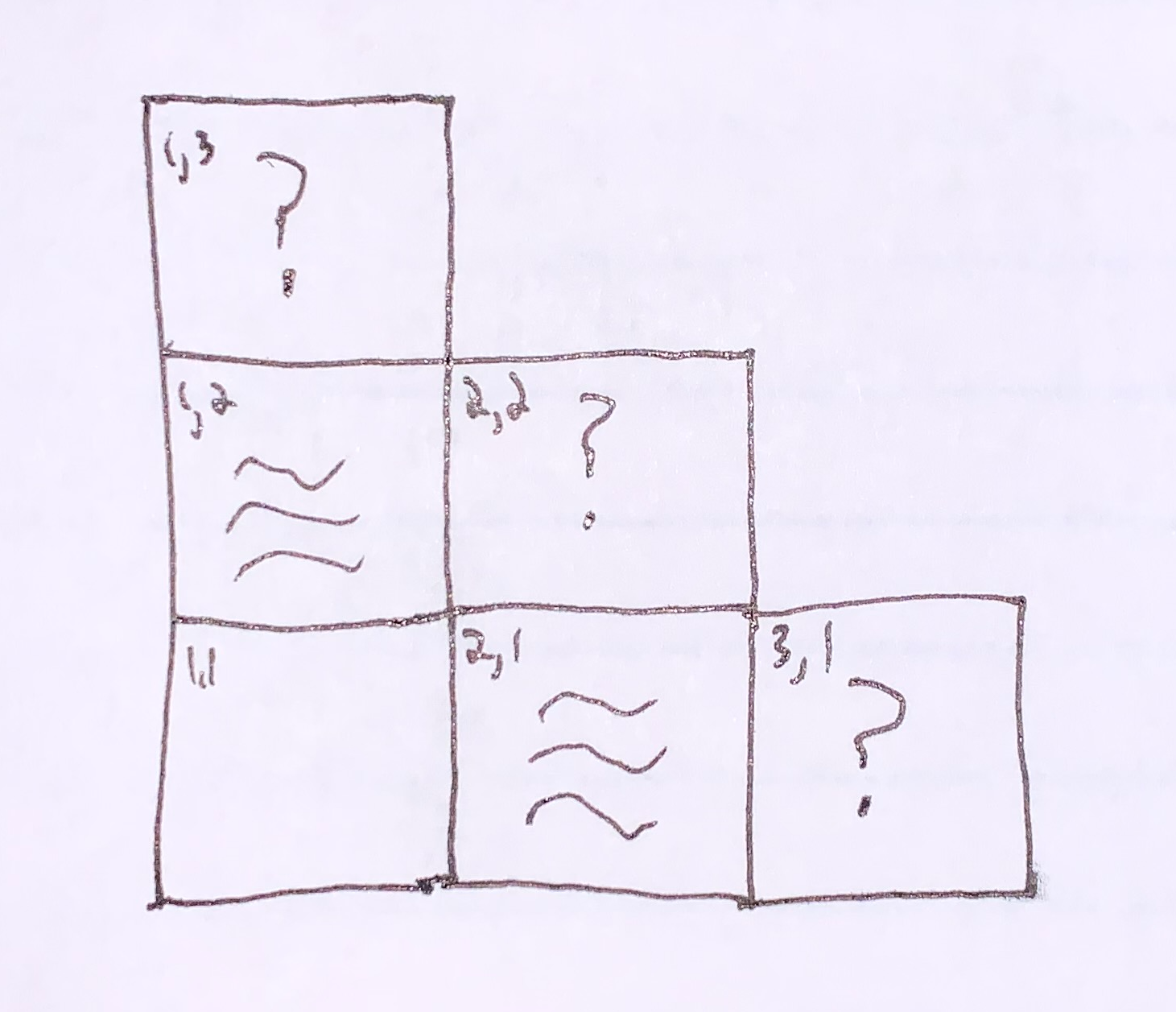
Possible pit configurations of [3,1], [2,2] and [3,1] (1 = pit, 0 = no pit):
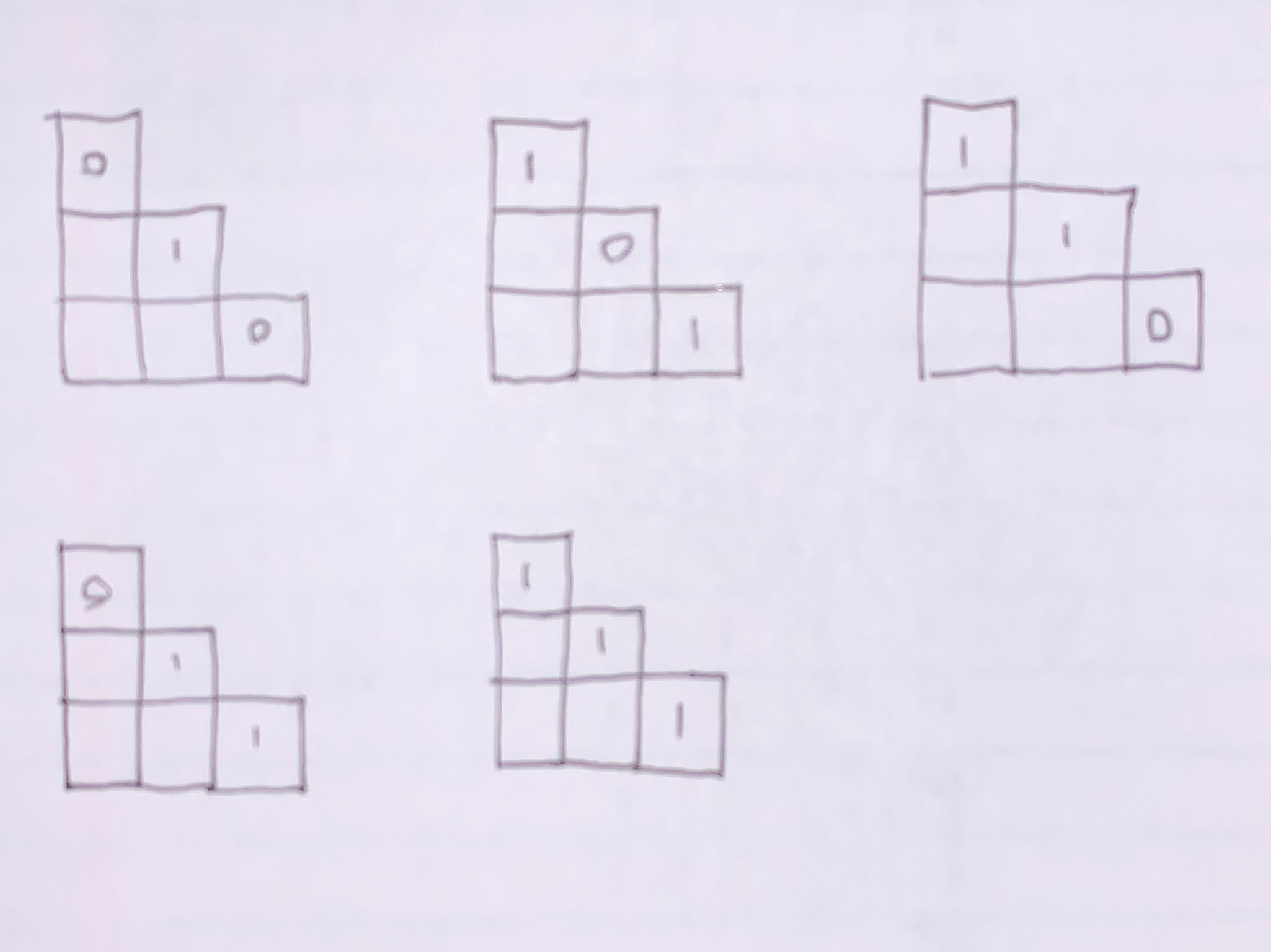
There are 10 remaining cells not depicted. Any pits not in [3,1], [2,2] and [3,1] will be in the remaining 10. Let’s count up the total number of states corresponding to each configuration:
| [1,3] | [2,2] | [3,1] | Count |
|---|---|---|---|
| 0 | 1 | 0 | ${10 \choose 2} = 45$ |
| 1 | 0 | 1 | ${10 \choose 1} = 10$ |
| 1 | 1 | 0 | ${10 \choose 1} = 10$ |
| 0 | 1 | 1 | ${10 \choose 1} = 10$ |
| 1 | 1 | 1 | ${10 \choose 0} = 1$ |
The total count is 76 states. As fractions (called probabilities), we have
$$
\begin{aligned}
p(0,1,0) &= 45/76 \\
p(1,0,1) &= 10/76 \\
p(1,1,0) &= 10/76 \\
p(0,1,1) &= 10/76 \\
p(1,1,1) &= 1/76
\end{aligned}
$$
The fraction of states where the middle cell [2,2] has a pit is $66/76$. The fraction of states where [3,1] has a pit is $21/76$, and likewise for [1,3]. We say that [2,2] is more likely to have a pit than [1,3] or [3,1]. If the agent is forced to choose one of the three cells to move to, [2,2] is the most dangerous option (highest probability of falling into a pit) and [3,1],[3,1] are equally less-dangerous.
The difference between the classical and Bayesian paradigms is now clear. A classical agent does not distinguish between these three options, since none of these cells can be proved to be pit-free (this property is not uniquely determined from the givens). The Bayesian agent doesn’t need unique determination to have knowledge about the pit-ness of these cells, and concludes that [2,2] is more likely to have a pit than [3,1] or [1,3].
Probability notation
$\newcommand{\obs}{\mathrm{Data}}$I’m now going to regard logical propositions as functions of state $\o$. For example, $R_1(\o)$ returns true if $\o$ is a math-model of proposition $R_1$, and false otherwise.
Let $\obs = R_1\and\dots\and R_5$. Then $\obs(\o)$ is true iff $\o$ is a math-model of our givens $R_1$ through $R_5$. If I write $P_{x,y}$, take that now to be a function of $\o$ as well.
Let $p$ be the uniform probability measure on $\O$. Using random variable notation (see zhat for probability theory and LW for conditional probability notation) the fraction of states where the middle cell [2,2] has a pit is $p(P_{2,2}=\1\mid\obs=\1) = 66/76$. The fraction of states where [3,1] and [1,3] have a pit respectively is $p(P_{1,3} = \1\mid\obs=\1) = p(P_{3,1} = \1\mid\obs=\1) = 21/76$.
In general for finite state sets $\O$, any ML-model $f : \O\to\X$ can be regarded as a random variable (or a tuple of random variables), i.e. a function from states to observables. I always assume a uniform probability measure, which corresponds to naive counting like in the example above. Let $f_{a:b}$ denote the slice of the tuple-valued random variable $f$ from index $a$ to $b$. Generally we want to determine the probability of some (unobserved) partial observation $x_{n:m}$ given the (observed) partial observation $x^*_{1:n}$:
$$
\begin{aligned}
& p(f_{n:m} = x_{n:m} \mid f_{1:n} = x^*_{1:n}) \\
&\quad= p\set{\o\in\O \mid f(\o) \in x^*_{1:n}`x_{n:m}} / p\set{\o\in\O \mid f(\o) \in x^*_{1:n}} \\
&\quad= p(\inv{f}(x^*_{1:n}`x_{n:m})) / p(\inv{f}(x^*_{1:n})) \\
&\quad= \abs{\inv{f}(x^*_{1:n}`x_{n:m})} / \abs{\inv{f}(x^*_{1:n})}
\end{aligned}
$$
Discussion
In general, the classically rational agent only regards uniquely determined partial observables (output dimensions on it’s ML-model $f$) as knowledge, and does not act on undetermined partial observables. In contrast, the Bayesian rational agent takes the relative proportion of possible states that produce each outcome as knowledge.
How does the Bayesian agent pull this off? Do these “Bayesian” probabilities really constitute knowledge? We can turn the question around and ask if uniquely determined observables really constitute knowledge. It is rare for something to be uniquely determined in practice. I suspect that many of the difficulties encountered in applications of statistical inference and machine learning are because of this. A classical reasoner needs to make simplifications and assumptions in service of being able to then uniquely determine something of interest. It seems to me that most of informal rational thought comes down to some version of choosing an ML-model s.t. something of interest can be uniquely determined. Described in this way, classical reasoning sounds biased. On the flip side, in practice Bayesian ML-models requires special simplifications and assumptions to be computationally tractable, so a similar sort of ML-model-choosing bias occurs.
Note that the size of $\O$ and the ML-model $f$ determine how many states produce each partial observation. Ostensibly these things are arbitrarily chosen by the agent. The classical reasoner objects that state-counts (probabilities) don’t constitute actual knowledge about the world, but are an artifact of the choice of ML-model $f$, and so it is inappropriate to treat these quantities as knowledge. The Bayesian reasoner counters that a classical ML-model (e.g. boolean logic) is also arbitrarily chosen. Unique determination is a property of $f$, not reality, and depends on the arbitrary simplifications and assumptions made by the agent. Thus, the Bayesian reasoner concludes, my approach is no less rational than yours.
The classical reasoner would counter that the parts of the ML-model output which are observed can be arbitrarily inspected for “goodness of fit” to reality. Unique determination is much less fragile (i.e. stable w.r.t. modeling inaccuracies) than state-counts. Unique determination is robust against worst-case modeling errors (though in practice this is clearly not true).
Punchline: any representation of the world whose predictions are not uniquely determined by data on hand can be viewed as Bayesian, if we are willing to provide a measure for calculating sizes of sets of model states, and then to use size-of-possibilities as decision making criteria.
The Bayesian Axiom
This epistemological debate is still raging. The efficacy of classical reasoning has been argued about for the last two and a half millennia. Bayesian reasoning is a more modern invention that, depending on how you count it, has been going on for 100 to 300 years (early 20th century Bayesians to Thomas Bayes). The frontier of contemporary inquery is the complex: from brains to human societies to high-dimensional physical systems, the neat and orderly unique-determination of classical reasoning is hard to come by. For this reason, Bayesian reasoning is gaining traction and is posturing to topple classical reasoning as the common-sense epistemological default.
Given the unsettled nature of these questions, it is my opinion that the “state-counts as knowledge” premise be taken as the “Bayesian axiom”. This neatly delineates classical and Bayesian epistemology down to one difference: Bayesian epistemology is classical epistemology plus an additional axiom. Some may accept this axiom and other’s may reject it, leading to different kinds of reasoning and knowledge. I don’t know if we will ever be able to determine that this axiom should or should not be used. In that case, like Euclid’s fifth axiom, “flat” and “curved” rationality shall forever remain parallel self-consistent options.