[This is an article, which is something I’ve optimized for readability and transmission of ideas, opposed to notes that are the seed of an idea and something I’ve written quickly.]

I will apply to abstract physics the same information algebra I introduced in Bayesian information theory and further developed in Information Algebra. Bayesian information is just information from the perspective of an agent that may have or not have particular information. Below, I will introduce the notion of a physical system having or not having information about itself or other systems (regardless of whether or not it has agenty attributes), and the same information algebra will apply. The only difference is a shift from the 1st person to 3rd person perspective.

$$
\newcommand{\0}{\mathrm{false}}
\newcommand{\1}{\mathrm{true}}
\newcommand{\mb}{\mathbb}
\newcommand{\mc}{\mathcal}
\newcommand{\mf}{\mathfrak}
\newcommand{\and}{\wedge}
\newcommand{\or}{\vee}
\newcommand{\es}{\emptyset}
\newcommand{\a}{\alpha}
\newcommand{\t}{\tau}
\newcommand{\T}{\Theta}
\newcommand{\D}{\Delta}
\newcommand{\o}{\omega}
\newcommand{\O}{\Omega}
\newcommand{\x}{\xi}
\newcommand{\z}{\zeta}
\newcommand{\fa}{\forall}
\newcommand{\ex}{\exists}
\newcommand{\X}{\mc{X}}
\newcommand{\Y}{\mc{Y}}
\newcommand{\Z}{\mc{Z}}
\newcommand{\P}{\Psi}
\newcommand{\y}{\psi}
\newcommand{\p}{\phi}
\newcommand{\l}{\lambda}
\newcommand{\B}{\mb{B}}
\newcommand{\m}{\times}
\newcommand{\N}{\mb{N}}
\newcommand{\R}{\mb{R}}
\newcommand{\I}{\mb{I}}
\newcommand{\H}{\mb{H}}
\newcommand{\e}{\varepsilon}
\newcommand{\Env}{\mf{E}}
\newcommand{\expt}[2]{\mb{E}_{#1}\left[#2\right]}
\newcommand{\set}[1]{\left\{#1\right\}}
\newcommand{\par}[1]{\left(#1\right)}
\newcommand{\vtup}[1]{\left\langle#1\right\rangle}
\newcommand{\abs}[1]{\left\lvert#1\right\rvert}
\newcommand{\inv}[1]{{#1}^{-1}}
\newcommand{\ceil}[1]{\left\lceil#1\right\rceil}
\newcommand{\dom}[1]{_{\mid #1}}
\newcommand{\df}{\overset{\mathrm{def}}{=}}
\newcommand{\M}{\mc{M}}
\newcommand{\up}[1]{^{(#1)}}
\newcommand{\Dt}{{\Delta t}}
\newcommand{\tr}{\rightarrowtail}
\newcommand{\tx}{\prec}
\newcommand{\qed}{\ \ \blacksquare}
\newcommand{\c}{\overline}
\newcommand{\A}{\mf{A}}
\newcommand{\cA}{\c{\mf{A}}}
\newcommand{\dg}{\dagger}
\newcommand{\lgfr}[2]{\lg\par{\frac{#1}{#2}}}
\newcommand{\rv}{\boldsymbol}
\require{cancel}
$$

$\newcommand{\sys}[2]{\left[#2\right]_{#1}}$

Information Preliminaries

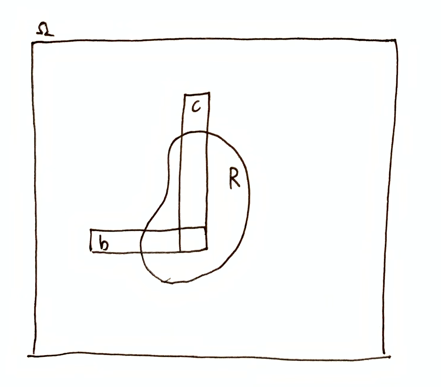
For sets $\O$ and $A \subseteq \O$,

$$
\O\tr A
$$

is information. This denotes the narrowing down of possibility space $\O$ to possibility space $A$ containing the true possibility $\o^*\in A$.

The information $\O\tr A$ implies a domain restriction. For some other set $B \subseteq \O$,

$$
B\dom{A} \df B \cap A
$$

is the domain restriction operation on $B$, which makes clear which set is the domain and which set is being restricted.

Let $\mf{P}$ be a partition of $\O$. Then

$$
\begin{aligned}
\mf{P}\dom{A} &\df \set{p\dom{A} \mid p\in\mf{P}} \\
&= \set{p\cap A \mid p\in\mf{P}}
\end{aligned}
$$

is the domain restriction of partition $\mf{P}$ to domain $A$, s.t. $\bigcup\mf{P} = A$.

Information Theory Of Systems

I will use the abstraction of physics that I introduced in Causality For Physics. Let $\O$ be a set of possible states and $\t_\Dt : \O\to\O$, $\Dt\in\R$, be a family of bijective time-evolution functions on $\O$. In general, time-evolution forms the group $(\set{\t_\Dt \mid \Dt\in\R}, \circ)$, where $\t_{\Dt+\Dt'} = \t_\Dt\circ\t_{\Dt'}$ and $\t_{-\Dt}=\t^{-1}_\Dt$, and $\t_0:\o\mapsto\o$ is the identity function.

I will regard $\O$ as the state-space of an entire universe (i.e. a closed system). The universe may contain any number of systems labeled “A”, “B”, “C”, etc., with respective state-spaces $A, B, C,\dots$, so that $\O\subseteq A\m B\m C\m \dots$ and states are tuples, $\o = (a, b, c, \dots) \in \O$. Then the time-evolution function

$$\t_\Dt : (a, b, c, \dots) \mapsto \t_\Dt(a, b, c, \dots)$$

jointly time-evolves all the systems simultaneously, which allows $\t_\Dt$ to incorporate arbitrary interactions between systems. This also means that the time evolution of, say, system A, depends on not just A’s state, but the state of all systems, i.e. the universe’s state $\o$.

There is an alternative way to describe systems using partitions. Let $\mf{A}, \mf{B}, \mf{C},\dots$ each be a partition on $\O$. Partition $\mc{A}$ is a representation of system A’s state space, partition $\mf{B}$ is a representation of system B’s state space, and so on. I’ll denote elements of a partition with lowercase letters, e.g. $a\in\mf{A},\ b\in\mf{B},\ c\in\mf{C},\ \dots$

In the state-space view, $a\in A$ is a featureless element of which universal states $\o$ are composed. In the partition view, on the other hand, $a\in\mf{A}$ is a subset of $\O$, corresponding to all the states of the universe that are indistinguishable to system A, i.e. the set of all universal states $\o\in\O$ for which system A is in the same state $a$. You can think of $\mf{A}$ as the set of equivalence classes for the relation “same state from system A’s perspective”. Let $\sys{\mf{A}}{\o}$ be the equivalence class containing $\o$, i.e. $\sys{\mf{A}}{\o} = a\in\mf{A}$ s.t. $\o\in a$.

From here on I will treat the states of systems as subsets of $\O$, and the state spaces of systems will be partitions of $\O$.

Systems Have Information

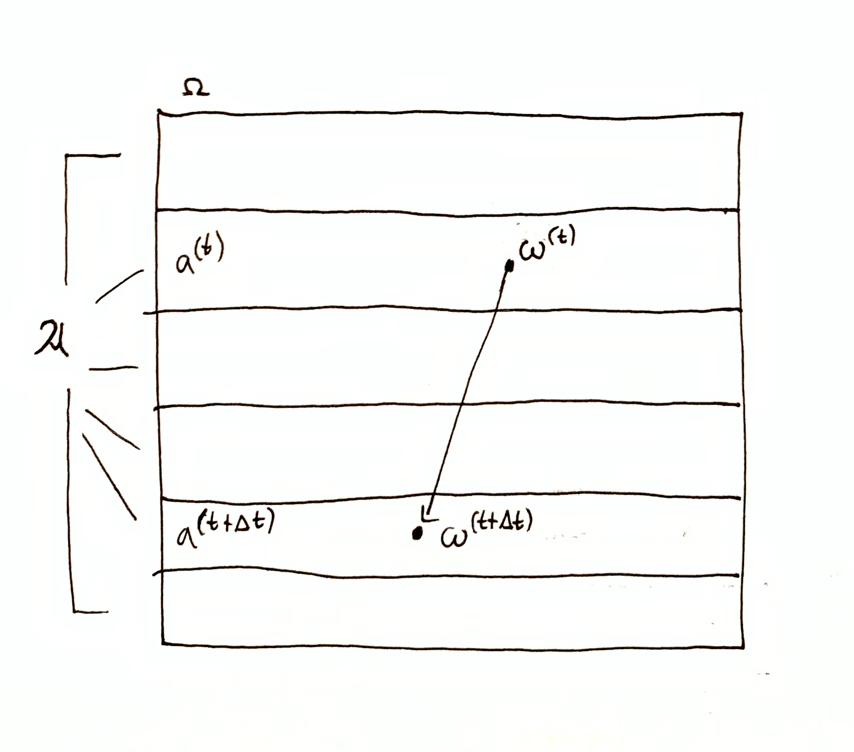
Suppose the universe is in state $\o\up{t}\in\O$ at time $t$. Then system A, with state space $\mf{A}$, is in state $a\up{t} = \sys{\mf{A}}{\o\up{t}}$. From system A’s perspective, $a\up{t}$ is the set of states the universe can be in.

System A has the information $\O \tr a\up{t}$, which reads “$\O$ is narrowed down to $a\up{t}$.” System A possesses this information in a purely physical sense. System A need not have awareness or understanding that it posses information, or even the capacity for awareness or understanding of anything. Merely as a physical description, I define any system with state space $\mf{A}$ to have the information $\O \tr \sys{\mf{A}}{\o\up{t}}$ at time $t$.

As a corollary, the universe has the information $\O\tr\set{\o\up{t}}$ at time $t$. The universe can be viewed as the supersystem with state space $\mf{O} = \set{\set{\o} \mid \o\in\O}$, the partition of singletons. In this sense, the universe has total information, corresponding to narrowing down to a single state.

This definition of what it means for a system to have information will allow us to talk about what information the system has about itself and other systems at various times, as well as the information the system gains or losses about them as time evolves.

Interactions

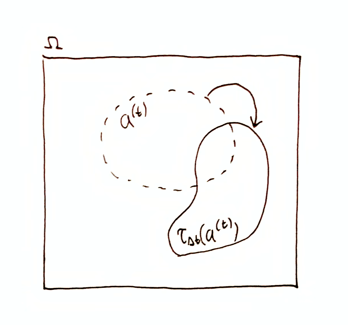
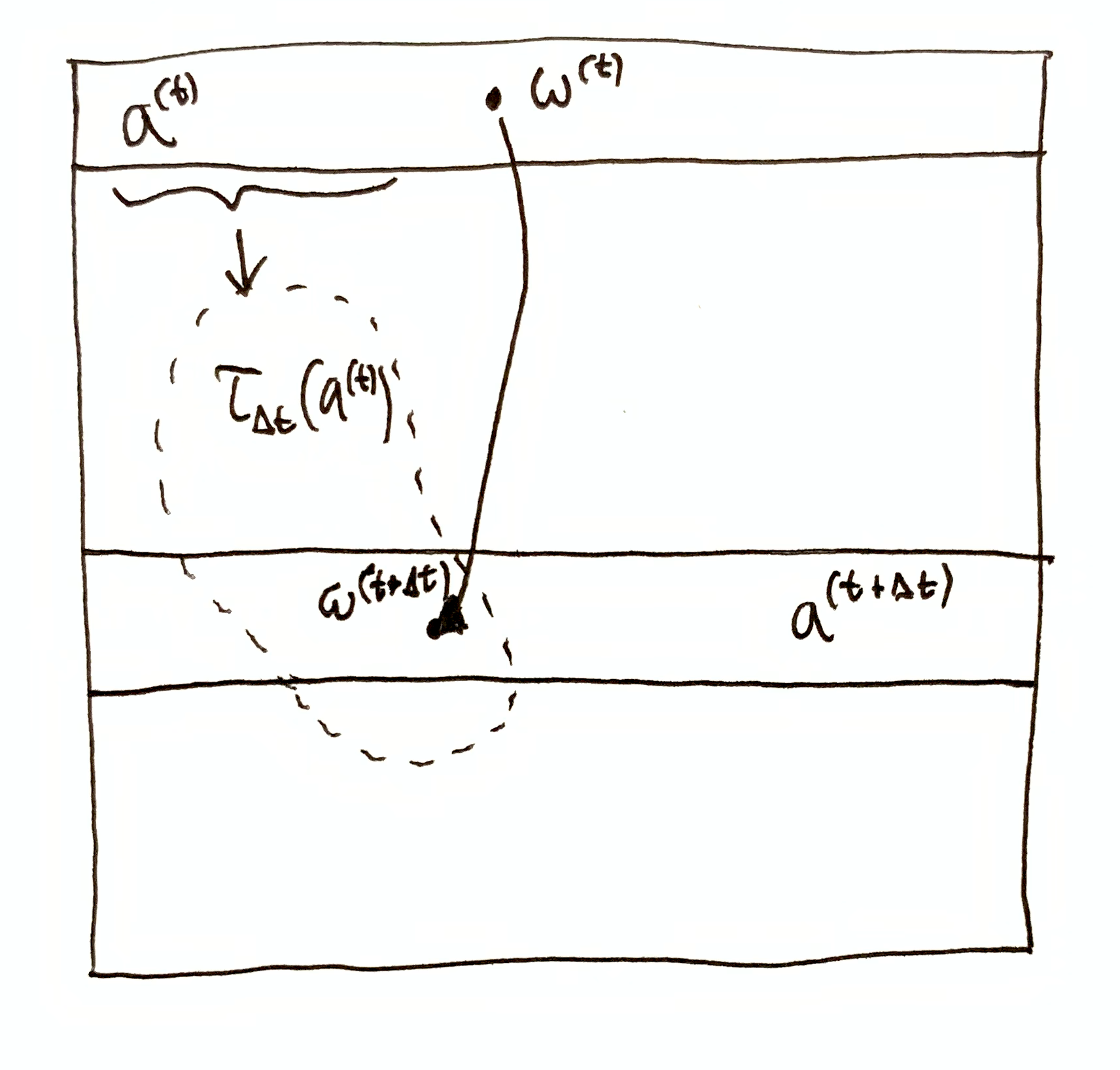
If $a\up{t}$ is the state of system A at time $t$, then $\t_{\Dt}(a\up{t})$ is NOT the time-evolution of system A’s state. A’s state at time $t+\Dt$ is $a\up{t+\Dt}=\sys{\mf{A}}{\o\up{t+\Dt}}$ where $\o\up{t+\Dt} = \t_\Dt(\o\up{t})$. If $\t_{\Dt}(a\up{t}) \neq a\up{t+\Dt}$, then system A interacted with another system (or the environment) in the time interval $(t, t+\Dt)$. Note that by necessity, $\o\up{t+\Dt} \in \t_{\Dt}(a\up{t})\cap a\up{t+\Dt}$.

Then what is $\t_{\Dt}(a\up{t})$? At time $t$, system A has information not just about time $t$, but about all other times. Specifically, at time $t$, system A has the information $\O\tr \t_{\Dt}(a\up{t})$ about time $t+\Dt$. It is important to distinguish between the time when a system has information and the time it has information about. So at time $t+\Dt$, system A has information $\O\tr \t_{-\Dt}(a\up{t+\Dt})$ about time $t$.

If $\t_{\Dt}(a\up{t}) \neq a\up{t+\Dt}$, then system A does not have complete information about its own future state, which is the necessary result of interaction. Furthermore, $\t_{\Dt}(a\up{t}) \neq a\up{t+\Dt} \iff \t_{-\Dt}(a\up{t+\Dt}) \neq a\up{t}$, and so after system A interacted, it has forgotten information about its previous state at time $t$. That is to say, interaction causes a system to lose information about its past.

Conservation Of Information

Recapping Information Algebra, suppose we are given some measure $\mu$ on $\O$. This measure need not be normalized. Then for measureable set $R\subseteq\O$, the quantity of the information $\O\tr R$ is given by

$$
h(\O\tr R) = h(R) = \lg\par{\frac{\mu(\O)}{\mu(R)}}\,,
$$

where $h(R)$ is the information content (or pointwise entropy) of $R$, and $h(\O\tr R)$ is my own shorthand notation to make it clear what information is being quantified.

Conservation of information is the property of any bijective time-evolution, whereby the information $\O\tr \t_\Dt(a\up{t})$ is enough to recover the information $\O\tr a\up{t}$, because $a\up{t} = \t^{-1}_\Dt(\t_\Dt(a\up{t}))$, for all $\Dt\in\R$. That is to say, time-evolution of arbitrary state sets $R\subseteq\O$ does not destroy the information $\O\tr R$ (this is distinct from the time-evolution of systems which, as we saw, can lose information).

Conservation of information quantity is a property of measure-preserving time-evolution. Let $\mu$ additionally be a $\t_\Dt$-invariant measure on $\O$, i.e. $\mu(\t_\Dt^{-1}(A)) = \mu(A)$ for all measurable $A\subseteq \O$ and for all $\Dt\in\R$. Because $\t_\Dt$ is bijective, this is equivalent to requiring $\mu(\t_\Dt(A)) = \mu(A)$. Then $h(\O\tr a\up{t}) = h(\O\tr \t_\Dt(a\up{t}))$ for all $t, \Dt\in\R$.

Conservation of information quantity is a stronger property that requires a $\t$-invariant measure in addition to bijective time-evolution. In classical mechanics, Liouville’s theorem shows that any Newtonian time-evolution preserves uniform measures on phase space. This result is sometimes referred to as conservation of information by physicists, who are referring to conservation of information quantity within my nomenclature. For details, see

• Liouville’s theorem - physicstravelguide.com (Davis & Schwichtenberg)
• Entropy and conservation of information - theoreticalminimum.com - (Susskind)
• On the Gibbs-Liouville theorem in classical mechanics (Henriksson)
• Hamiltonian mechanics is conservation of information entropy (Carcassi & Aidala)

Information About Systems

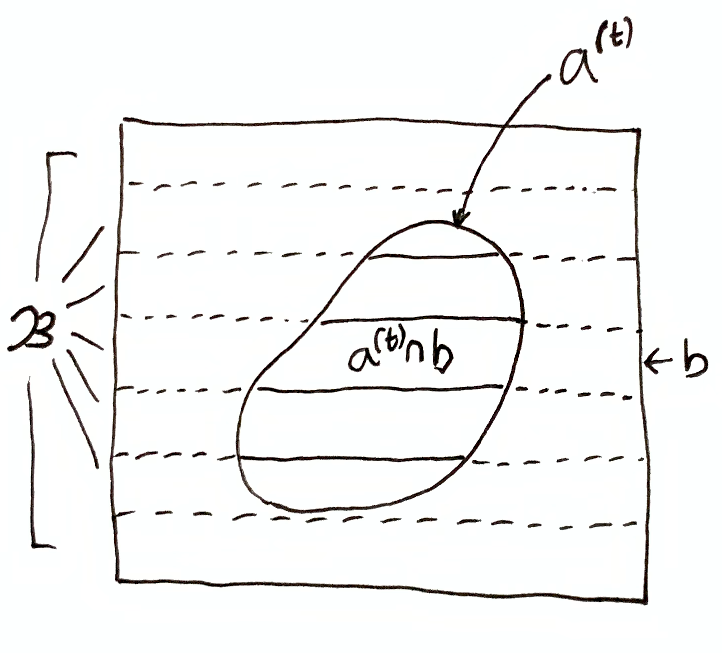
Suppose there are at least two systems, A and B, with respective state spaces $\mf{A}$ and $\mf{B}$. Let system A be in state $a\up{t}$ at time $t$. System A (at $t$) has the information $\O\tr \t_{\Dt}(a\up{t})$ about time $t+\Dt$. What information does A have about B’s state at time $t+\Dt$?

In Information Algebra, I showed that pointwise mutual information (PMI) quantifies “information about”. Specifically,

$$
i(a\up{t}, b) = i(b, a\up{t}) = \lg\par{\frac{\mu(a\up{t}\cap b)\mu(\O)}{\mu(a\up{t})\mu(b)}}
$$

quantifies how much information system A, being in state $a\up{t}$, has about whether system B is in state $b\in\mf{B}$ at time $t$.

If $i(a\up{t}, b) = 0$, then $a\up{t}$ and $b$ are orthogonal states. State spaces $\mf{A}$ and $\mf{B}$ are called orthogonal iff $i(a,b) = 0$ for all $a\in\mf{A}$ and $b\in\mf{B}$. Usually, systems are defined to be orthogonal, meaning that the state of one system can be chosen totally independently of the state of the other. Non-orthogonal systems have information about each other by construction, regardless of their mutual time-evolution. On the other hand, orthogonal systems always have zero information about each other at the present moment. That is to say, $i(a\up{t}, b) = 0$ for all $\mf{B}$, i.e. system A has no information about the state of system B at time $t$. However, system A may have information about system B’s past or future state.

$\O\tr \t_\Dt(a\up{t})$ is the information system A has at time $t$ about time $t+\Dt$. Then it follows that $i(\t_\Dt(a\up{t}), b)$ is the quantity of information system A has, at time $t$, about whether system B is in state $b$ at time $t+\Dt$. If $\t_\Dt(a\up{t}) \in b$, then $i(\t_\Dt(a\up{t}), b) = h(b) = h(\O\tr b)$ and system A (at time $t$) has certainty that system B is in state $b$ at time $t+\Dt$. On the other hand, if $b \in \t_\Dt(a\up{t})$, then $i(\t_\Dt(a\up{t}), b) = h(\t_\Dt(a\up{t})) = h(\O\tr \t_\Dt(a\up{t}))$ which is just the total quantity of information that system A has about time $t+\Dt$.

To fully lay out what information system A has (at time $t$) about system B’s state at time $t+\Dt$, we need to look at all the quantities of information A has about every state $b\in\mf{B}$, which can be given as the vector

$$
\vtup{i(\t_\Dt(a\up{t}), b) \mid b\in\mf{B}}\,.
$$

Note that $i(\t_\Dt(a\up{t}), b)$ can be negative (and has no lower bound), which means that system A has needs more quantity of information than $h(\O\tr b)$ to have certainty that system B is in state $b$. If system A has information that rules out state $b$ with certainty, i.e. $b\cap \t_\Dt(a\up{t}) = \es$, then $i(\t_\Dt(a\up{t}), b) = -\infty$. Information Algebra goes into further detail about the interpretation of PMI quantities.

Information Gain

The difference

$$
i(\t_{t'-t-\Dt}(a\up{t+\Dt}), b) - i(\t_{t'-t}(a\up{t}), b)
$$

is information gain, i.e. the information system A gained (or lost if negative) about whether system B is in state $b$ at time $t'$ due to the time-evolution of system A’s state over the time interval $(t,t+\Dt)$.

Likewise, $i(\t_{t'-t-\Dt}(a\up{t+\Dt}), a) - i(\t_{t'-t}(a\up{t}), a)$ is system A’s information gain (or loss) about itself, specifically whether it is in state $a$ at time $t'$.

Sum-Conservation Laws

Let $\O\tr R$ be the information some unspecified system at some unspecified time has about some other time. Then that system has the quantity of information $h(\O\tr R)$.

Let $b\in\mf{B}$ be a possible state of system B. Suppose $i(b, R) < h(\O\tr R)$. Then you might ask, “where did the remaining information go?” That is to say, does it make sense to think that the complete quantity of information $h(\O\tr R)$ should be divided among information about various things? Could we then have the information about everything add up to $h(\O\tr R)$, analogous to how conservation of mass and energy in physics results in reactions or interactions s.t. the energies and masses of the outputs add up to the input energy and mass?

Information does not quite work like this. For instance, the sum of the vector $\vtup{i(\t_\Dt(a\up{t}), b) \mid b\in\mf{B}}$ need not be $h(R)$. This is evident when you consider that it’s possible for the system with information $\O\tr R$ to have the information quantity $h(R)$ about $b\in\mf{B}$ and about $b'\in\mf{B}$, if both $b$ and $b'$ are contained within $R$. Then at least two entries in the vector are each $h(R)$. Furthermore, entries can be arbitrarily negative, and even $-\infty$ as we saw above.

I have found two ways to achieve something like a sum-conservation law for information quantity. One way uses pointwise quantities, and the other way uses expected quantities, i.e. entropy and mutual information.

Pointwise

Suppose $i(b, R) < h(\O\tr R)$. If we “shrank” $b$ down by intersecting with some other set $c$ such that $b \cap c \subseteq R$, then we’d have $i(b\cap c, R) = h(\O\tr R)$. Writing $i(b\cap c, R)$ as a sum involving $i(b, R)$ gives us a sum-conservation law:

$$
\begin{aligned}
i(b \cap c, R) &= i(b, R) + i(c, R) - i(b, c, R) \\
&= i(b, R) + i(c, R) - i(b, c) + i(b, c \mid R) \\
&= h(\O\tr R)\,.
\end{aligned}
$$

This is easy to check using the definition of PMI and $i(b, c, R)\df i(b, c) - i(b, c \mid R)$, and

$$
i(b, c \mid R) \df \lg\par{\frac{\mu(b\cap c\cap R)\mu(R)}{\mu(b\cap R)\mu(c \cap R)}}\,.
$$

If $c$ is chosen such that $b$ and $c$ are orthogonal, i.e. $i(b,c)=0$, and plugging in $h(\O\tr R)$ for $i(b \cap c, R)$, then we have the simpler form

$$
h(\O\tr R) = i(b, R) + i(c, R) + i(b, c \mid R)\,,
$$

which does not involve the information quantity $i(b,c)$ due to redundancy between the choice of $b$ and $c$.

Note that the “$i$” quantities may be negative, but $h(\O\tr R)$ is always positive. Thus at least one of these terms is positive.

It is possible for the information $\O\tr R$ to not contain information (or contain negative information) about $b$ or $c$. Then all of the positive information quantity goes into the term $i(b, c \mid R)$, which can be thought of as the quantity of information $\O\tr b$ has about whether $c$ is the case, given the smaller state space $R$.

Information about more than two sets

Suppose $i(b\cap c, R) < h(\O\tr R)$. We can repeat the process above again by choosing a third set $a$ s.t. $i(a\cap b\cap c, R) = h(\O\tr R)$. In general, there is an $n$-way relationship.

Let $x_1,\dots,x_n,R \subseteq \O$ be arbitrary sets. Then,

$$
i(x_1\cap\dots\cap x_n,R) = i(x_1\cap\dots\cap x_{n-1},R) + i(x_n, R \mid x_1\cap\dots\cap x_{n-1})\,.
$$

Using the identity

$$
\begin{aligned}
& i(y_{n-k+1}, \dots, y_n, R \mid y_1\cap\dots\cap y_{n-k}) \\
&\quad\,\, = \,\,i(y_{n-k+1}, \dots, y_n, R \mid y_1\cap\dots\cap y_{n-k-1}) \\
&\qquad\quad- i(y_{n-k}, \dots, y_n, R \mid y_1\cap\dots\cap y_{n-k-1})
\end{aligned}
$$

we can recursively expanding out these terms to produce an expression for $i(x_1\cap\dots\cap x_n,R)$ entirely composed of non-conditional multi-way PMI terms of the form $i(y_1, \dots, y_n)$.

So for example, expanding out $i(x_n, R \mid x_1\cap\dots\cap x_{n-1})$ with $k=1$, we have

$$
\begin{aligned}
& i(x_n, R \mid x_1\cap\dots\cap x_{n-1}) \\
&\quad=\,\, i(x_n, R \mid x_1\cap\dots\cap x_{n-2}) \\
&\qquad\,\,- i(x_{n-1}, x_n, R \mid x_1\cap\dots\cap x_{n-2})\,.
\end{aligned}
$$

Then further expanding out the resulting terms, using $y_1, \dots, y_{n'} = x_1, \dots, x_{n-2}, x_n$ and $k=1$, we get

$$
\begin{aligned}
& i(x_n, R \mid x_1\cap\dots\cap x_{n-2})\\
&\quad=\,\, i(x_n, R \mid x_1\cap\dots\cap x_{n-3}) \\
&\qquad\,\,- i(x_{n-2}, x_n, R \mid x_1\cap\dots\cap x_{n-3})\,,
\end{aligned}
$$

and using $y_1, \dots, y_n = x_1, \dots, x_n$ and $k=2$, we get

$$
\begin{aligned}
& i(x_{n-1}, x_n, R \mid x_1\cap\dots\cap x_{n-2}) \\
&\quad=\,\, i(x_{n-1}, x_n, R \mid x_1\cap\dots\cap x_{n-3}) \\
&\qquad\,\,- i(x_{n-2}, x_{n-1}, x_n, R \mid x_1\cap\dots\cap x_{n-3})\,.
\end{aligned}
$$

Repeat this process of expanding out these terms until all conditional arguments are gone.

Multi-way PMI terms can then be converted into 2-way PMI terms using the definition $i(y_1, \dots, y_n) \df i(y_1, \dots, y_{n-1}) - i(y_1, \dots, y_{n-1}\mid y_n)$.

For case of three sets $a,b,c$, we have

$$
\begin{aligned}
& i(a\cap b\cap c,R) \\
&\quad\,=\, i(a, R) + i(b, R) + i(c, R) \\
&\qquad\,\,- i(a, b, R) - i(a, c, R) - i(b, c, R) \\
&\qquad\,\,+ i(a,b,c,R)
\end{aligned}
$$

where

$$
\begin{aligned}
i(a,b,c,R) &= i(a,b,c) - i(a,b,c\mid R)\\
&= i(a,b) - i(a,b \mid c) - i(a,b \mid R) + i(a,b \mid c\cap R)\,.
\end{aligned}
$$

If $a,b,c$ are all mutually orthogonal, i.e. $i(a,b) = i(a,c) = i(b,c) = i(a,b,c) = 0$, then

$$
\begin{aligned}
& i(a\cap b\cap c,R) \\
&\quad\,=\, i(a, R) + i(b, R) + i(c, R) \\
&\qquad\,\,+ i(a,b \mid R) + i(b,c \mid R) + i(a,b \mid c\cap R)\,.
\end{aligned}
$$

Expectation

It would be nice if there was a single quantity describing $\mf{B}\tr\mf{B}\dom{R}$, the narrowing down of partition $\mf{B}$ to domain $R$, analogous to $h(\O\tr R)$ for individual sets. I will motivate such a quantity from a few special cases.

If $P\subseteq 2^\O$ is some set of sets, then let $\mu(P) = \mu(\bigcup P)$. Then for partition $\mf{B}$ of $\O$, we have $\mu(\mf{B}) = \mu(\bigcup\mf{B}) = \mu(\O)$. Let’s define the quantity $h(\mf{B}\tr \mf{B}\dom{R})$ on a few special cases.

Consider $\mf{B}\tr \set{b}$ for some $b\in\mf{B}$.

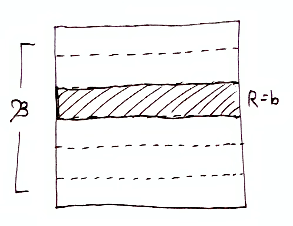
Let

$$
\begin{aligned}
h(\mf{B}\tr \set{b}) &= \lg\par{\frac{\mu(\mf{B})}{\mu\set{b}}} \\
&= \lg\par{\frac{\mu(\O)}{\mu(b)}} \\
&= h(\O\tr b)\,.
\end{aligned}
$$

Then the quantity of information due to narrowing down the partition $\mf{B}$ to one of its elements $b$ is equal to the quantity of information due to narrowing down the possibility space $\O$ to $b$.

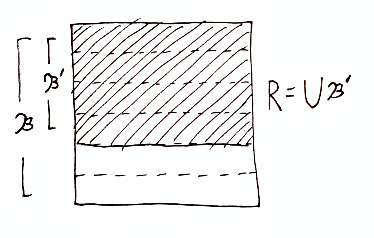
In general, let $\mf{B}' \subseteq \mf{B}$. Then

$$
\begin{aligned}
h(\mf{B}\tr \mf{B}') &= \lg\par{\frac{\mu(\mf{B})}{\mu(\mf{B}')}} \\
&= \lg\par{\frac{\mu(\O)}{\mu(\bigcup \mf{B}')}} \\
&= h\par{\O\tr \bigcup \mf{B}'}\,.
\end{aligned}
$$

One more special case: suppose $\mf{B}$ and $\mf{B}\dom{R}$ are uniform, meaning that $\mu(b) = \mu(b')$ or $0$ for all $b,b'\in\mf{B}$, and likewise for $\mf{B}\dom{R}$ (which may contain the empty set).

Then

$$
\begin{aligned}
h(\mf{B}\tr \mf{B}\dom{R}) &= h(\O\tr b) - h(R \tr b\cap R)\\
&= h(\O\tr R) - h(b \tr b\cap R)\\
&= i(b, \bigcup \mf{B}\dom{R}) \\
&= i(b, R)
\end{aligned}
$$

for some $b\in\mf{B}$ s.t. $b\cap R \neq \es$. If $R$ reduces each $b\in\mf{B}$ by the same amount, then $i(b, R) = 0$ for all $b\in\mf{B}$ (i.e. $R$ and $b$ are orthogonal), and so $h(\mf{B}\tr \mf{B}\dom{R}) = 0$, indicating that $\O\tr R$ contains no information about the partition $\mf{B}$.

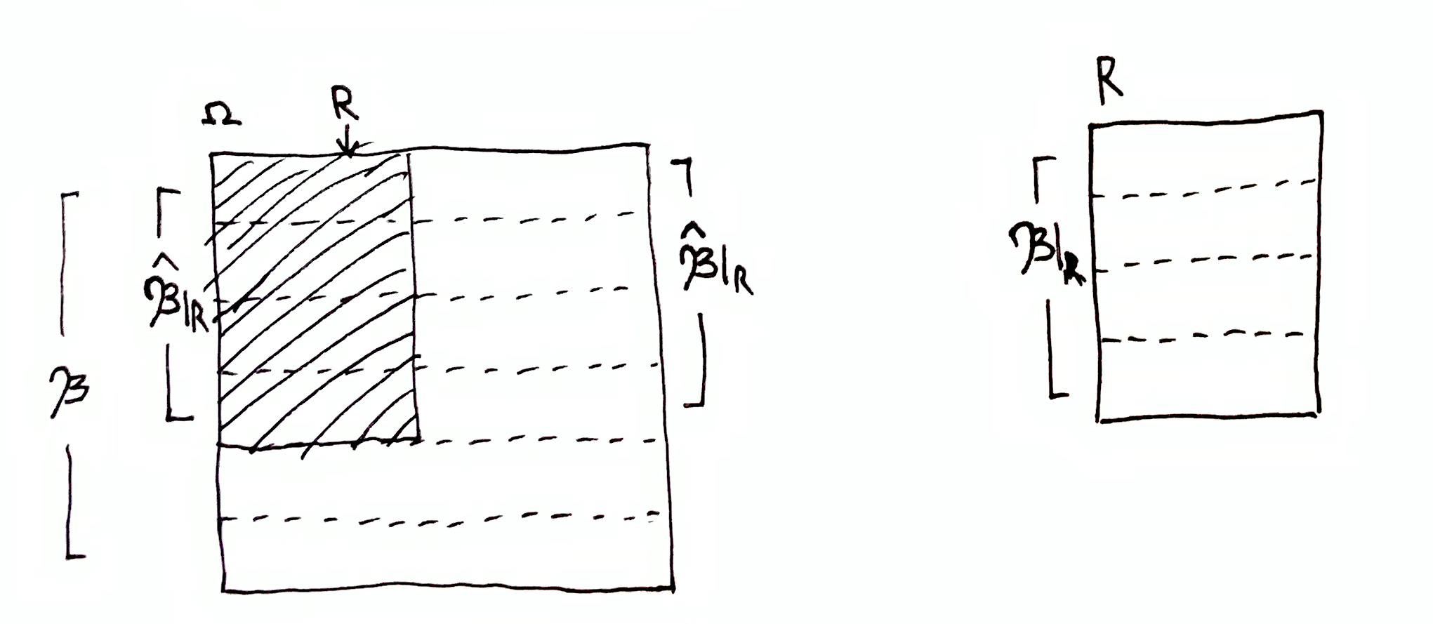
Let $\hat{\mf{B}}\dom{R} = \set{b\in\mf{B} \mid b\cap R \neq \es}$ be the subset of $\mf{B}$ containing elements that have non-zero intersection with $R$. We’d like $h(\mf{B}\tr \mf{B}\dom{R}) = h(\mf{B}\tr \hat{\mf{B}}\dom{R}) = \lg\par{\frac{\mu(\mf{B})}{\mu(\hat{\mf{B}}\dom{R})}}$. Notice that $\mu(b)/\mu(\bigcup\hat{\mf{B}}\dom{R}) = \mu(b\cap R)/\mu(R)$, which gives us

$$
\mu(\bigcup\hat{\mf{B}}\dom{R}) = \mu(b)\frac{\mu(R)}{\mu(b\cap R)}\,.
$$

Plugging in, we get $\lg\par{\frac{\mu(\mf{B})}{\mu(\hat{\mf{B}}\dom{R})}} = \lg\par{\frac{\mu(\O)}{\mu(b)\frac{\mu(R)}{\mu(b\cap R)}}} = i(b, R)$.

Mutual Information

In the more general case $\mf{B}$ and $\mf{B}\dom{R}$ are not uniform partitions. We will need some kind of averaging operation over $i(b,R)$ for $b\in\mf{B}$ that reduces to our special cases above, and zeros out all the $i(b,R) = -\infty$ terms where $b\cap R = \es$. Taking the expectation w.r.t. $\mu(\cdot \mid R)$ fulfills both requirements.

Let

$$
\expt{x\in\mf{X}}{f(x)} = \frac{1}{\mu(\bigcup\mf{X})} \sum_{x\in\mf{X}} \mu(x)\,f(b)
$$

for discrete $\mf{X}$ and

$$
\expt{x\in\mf{X}}{f(x)} = \frac{1}{\mu(\bigcup\mf{X})}\int_{x\in\mf{X}} \rho(x)\,f(b)\,\mathrm{d}x
$$

for continuous $\mf{X}$, where $\rho$ is the density function for measure $\mu$. These quantities are normalized by $\mu(\bigcup\mf{X})$ where $\bigcup\mf{X}$ is the domain of the partition $\mf{X}$.

Define the mutual information between partitions $\mf{A}$ and $\mf{B}$ as

$$
\I(\mf{A}, \mf{B}) \df \expt{a\in\mf{A},b\in\mf{B}}{i(a,b)}\,,
$$

as well as the conditional mutual information

$$
\I(\mf{A}, \mf{B} \mid R) \df \expt{a\dom{R}\in\mf{A}\dom{R},b\dom{R}\in\mf{B}\dom{R}}{i(a,b\mid R)}\,.
$$

Define the mutual information between partition $\mf{B}$ and set $R$ as

$$
\I(\mf{B}, R) \df \expt{b\dom{R}\in\mf{B}\dom{R}}{i(b,R)}\,.
$$

In the discrete case,

$$
\I(\mf{B}, R) = \sum_{b\in\mf{B}} \frac{\mu(b\cap R)}{\mu(R)}i(b,R)\,.
$$

In general, define the quantity of information that $\O\tr R$ contains about which element of partition $\mf{B}$ is the state of system B:

$$
h(\mf{B}\tr \mf{B}\dom{R}) \df \I(\mf{B}, R)\,.
$$

Let $\mf{C}$ be the state space of some other system C. Taking the expectation of the pointwise sum-conservation law from above, we get

$$
\begin{aligned}
\I(\mf{B}\otimes\mf{C}, R) &= \I(\mf{B}, R) + \I(\mf{C}, R) - \I(\mf{B}, \mf{C}, R) \\
&= \I(\mf{B}, R) + \I(\mf{C}, R) - \I(\mf{B}, \mf{C}) + \I(\mf{B}, \mf{C} \mid R)\,,
\end{aligned}
$$

where

$$
\mf{B}\otimes\mf{C}\df \set{b\cap c \mid b\in\mf{B} \and c\in\mf{C}}
$$

is the partition product of $\mf{B}$ and $\mf{C}$, i.e. the intersection of all pairs of elements of $\mf{B}$ and $\mf{C}$.

While $\I(\mf{B}, R)$ and $\I(\mf{C}, R)$ are always non-negative (2-way mutual information is always non-negative), the 3-way mutual information $\I(\mf{B}, \mf{C}, R)$ can be negative. If $\mf{B}$ and $\mf{C}$ are orthogonal, i.e. $\I(\mf{B}, \mf{C}) = 0$, then

$$
\I(\mf{B}\otimes\mf{C}, R) = \I(\mf{B}, R) + \I(\mf{C}, R) + \I(\mf{B}, \mf{C} \mid R)\,,
$$

which is a decomposition of $\I(\mf{B}\otimes\mf{C}, R)$ into non-negative terms. This looks more like the sum-conservation laws we have for mass and energy (sum of non-negative terms is conserved).

Environments

Let $\mf{B}$ be some state space. A partition complement of $\mf{B}$, denoted $\c{\mf{B}}$, satisfies the following properties:

0. $\c{\mf{B}}$ is a partition of $\O$.
1. $\I(\mf{B}, \c{\mf{B}}) = 0$,
2. $\mf{B}\otimes\c{\mf{B}} = \mf{O} = \set{\set{\o}\mid\o\in\O}$.

In general, $\mf{B}$ does not have a unique complement, and may not have any complement. For example, if $\O = \set{\o_1, \o_2, \o_3}$ and $\mf{B} = \set{\set{\o_1, \o_2}, \set{\o_3}}$, then it is easy to check that $\mf{B}$ has no complement.

If each element of $\mf{B}$ is infinite, then $\mf{B}$ always has a complement. If each element of $\mf{B}$ is finite, then it has a complement if each element has the same cardinality.

We can regard a complement $\c{\mf{B}}$ as the environment of system B, which is everything in the universe outside of system B.

Assuming $\mf{B}$ has a complement $\c{\mf{B}}$, then the sum-conservation law from above is

$$
\I(\mf{B}\otimes\c{\mf{B}}, R) = \I(\mf{B}, R) + \I(\c{\mf{B}}, R) + \I(\mf{B}, \c{\mf{B}} \mid R)\,.
$$

A useful identity here is that $\I(\mf{O}, R) = h(\O\tr R)$. Since $\mf{B}\otimes\c{\mf{B}} = \mf{O}$, then we have

$$
h(\O\tr R) = \I(\mf{B}, R) + \I(\c{\mf{B}}, R) + \I(\mf{B}, \c{\mf{B}} \mid R)\,.
$$

Proof that $\I(\mf{O}, R) = h(\O\tr R)$.

Let $\mf{X}$ be a partition of $\O$ s.t. for each $x\in\mf{X}$, either $x\cap R = \es$ or $x$. That is to say, there is some subset $Y \subseteq \mf{X}$ s.t. $R = \bigcup Y$. Then $Y = \mf{X}\dom{R}$.

$$
\begin{aligned}
\I(\mf{X}, R) &= \sum_{x\in\mf{X}} \mu(x \mid R) \lg\par{\frac{\mu(x\cap R)\mu(\O)}{\mu(x)\mu(R)}} \\
&= \sum_{x\in \mf{X}\dom{R}} \mu(x \mid R) \lg\par{\frac{\cancel{\mu(x)}\mu(\O)}{\cancel{\mu(x)}\mu(R)}} \\
&= \lg\par{\frac{\mu(\O)}{\mu(R)}} \\
&= h(\O\tr R)\,.
\end{aligned}
$$

Since $\mf{O}$ is the singleton partition, it satisfies the condition above for all $R\subseteq \O$. Thus $\I(\mf{O}, R) = h(\O\tr R)$. $\qed$

Combining conservation of information quantity,

$$
h(\O\tr R) = h(\O\tr \t_\Dt(R))\,,
$$

with the sum-conservation law, we get

$$
\begin{aligned}
& \I(\mf{B}, R) + \I(\c{\mf{B}}, R) + \I(\mf{B}, \c{\mf{B}} \mid R) \\
=\,\, & \I(\mf{B}, \t_\Dt(R)) + \I(\c{\mf{B}}, \t_\Dt(R)) + \I(\mf{B}, \c{\mf{B}} \mid \t_\Dt(R))\,.
\end{aligned}
$$

Consider system A with state space $\A$, and its environment with state space $\cA$. At time $t$, system A is in state $a\up{t}\in\mf{A}$ and has the information $\O\tr a\up{t}$ about time $t$. Since $\I(\A, a\up{t}) = h(\O\tr a\up{t})$, then $\I(\cA, a\up{t}) + \I(\A, \cA \mid a\up{t}) = 0$.

Then our conservation law reduces to

$$
\begin{aligned}
\I(\A, a\up{t}) &= \I(\A, \t_\Dt(a\up{t})) + \I(\cA, \t_\Dt(a\up{t})) + \I(\A, \cA \mid \t_\Dt(a\up{t})) \\
&= h(\O\tr a\up{t}) \,.
\end{aligned}
$$

If $\I(\A, \t_\Dt(a\up{t})) = h(\O\tr \t_\Dt(a\up{t})) = h(\O\tr a\up{t})$, then $\I(\cA, \t_\Dt(a\up{t})) + \I(\A, \cA \mid \t_\Dt(a\up{t})) = 0$ and system A (at time $t$) has no information about the environment at time $t+\Dt$. Since all the terms are positive, for system A to have information about the future environment, system A must have less than complete information about its own future state.

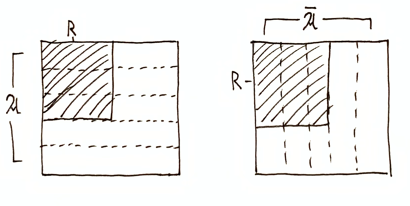
A tricky case to be aware of is when $\I(\A, \t_\Dt(a\up{t})) = 0$ and $\I(\cA, \t_\Dt(a\up{t})) = 0$. This would seem to be saying that system A has no information about its own future state and the environment’s future state. It would then seem that the information quantity $h(\O\tr a\up{t})$ simply disappeared and was not conserved. That quantity went into the third term, $\I(\A, \cA \mid \t_\Dt(a\up{t})) = h(\O\tr a\up{t})$, which indicates that system A becomes highly correlated with its environment in the future.

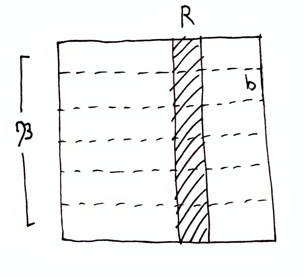
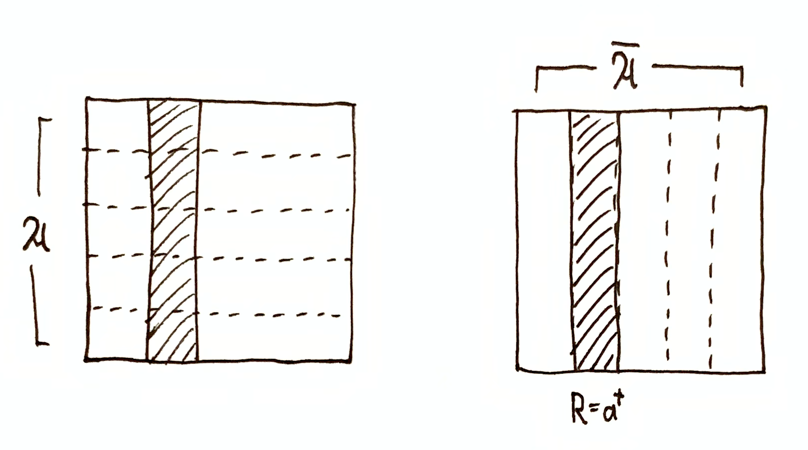
$R=a\in\A$. Then $\I(\A,R) = h(\O\tr R)$ and $\I(\cA,R) = 0$, $\I(\A,\cA \mid R) = 0$.

$R=a^\dg\in\cA$. Then $\I(\cA,R) = h(\O\tr R)$ and $\I(\A,R) = 0$, $\I(\A,\cA \mid R) = 0$.

$\I(\A,R)$ and $\I(\cA,R)$ are both non-zero, and $\I(\A,\cA \mid R) = 0$, meaning $\A$ and $\cA$ are still orthogonal when restricted to the domain $R$.

$\I(\A,R) = 0$ and $\I(\cA,R) = 0$, since restricting either partition to the domain $R$ still tells you nothing about the other partition. However, $\I(\A,\cA \mid R) = h(\O\tr R)$, meaning $\A$ and $\cA$ restricted to the domain $R$ are maximally redundant, i.e. given $R$ and some $a\in\mf{A}$, you can uniquely determine $a^\dg\in\mf{A}$, and vice versa.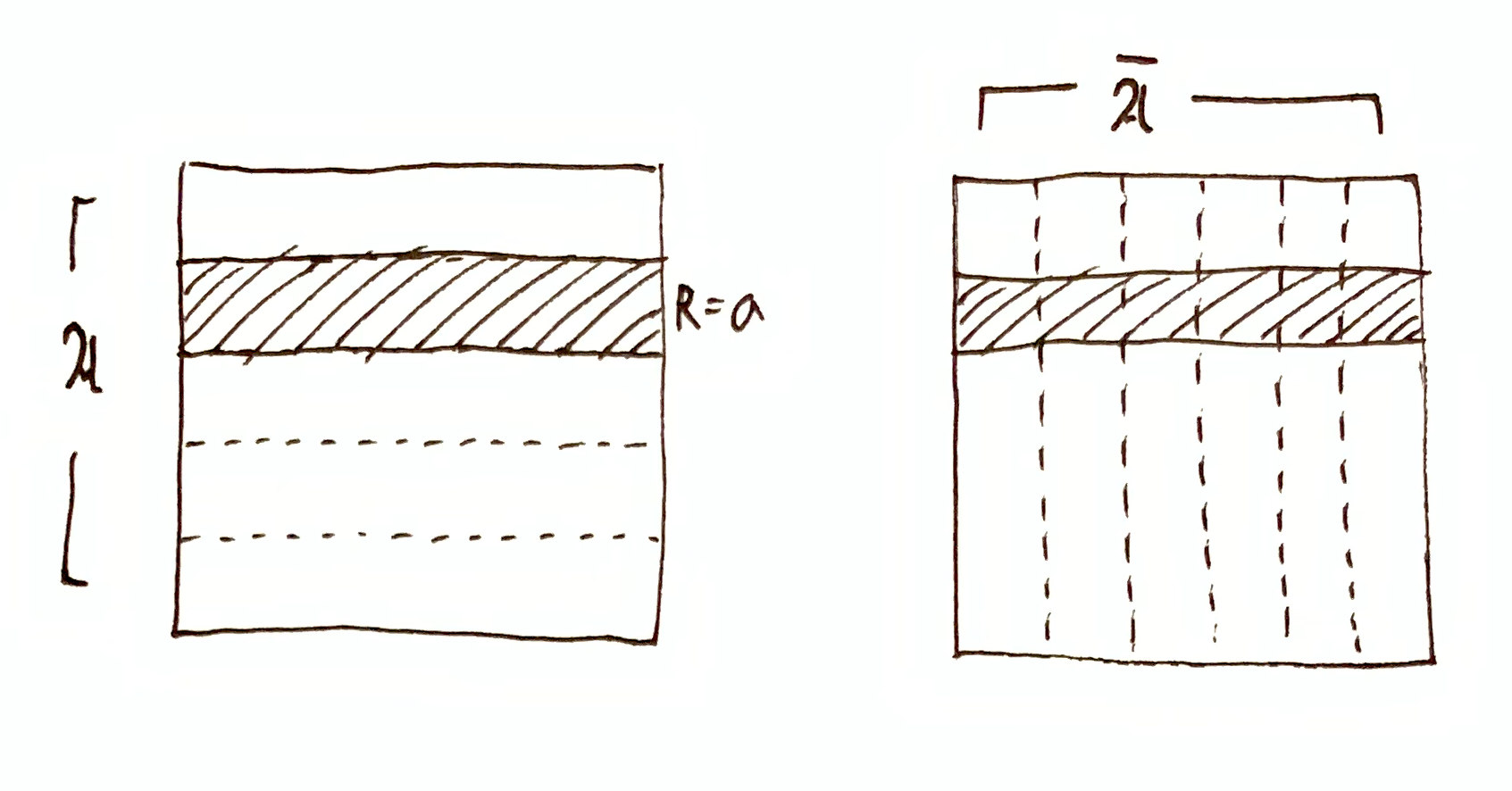

General Case

For arbitrary systems with state spaces $\A$ and $\mf{B}$, we have

$$
\I(\A\otimes\mf{B}, R) = \I(\A, R) + \I(\mf{B}, R) + \I(\A, \mf{B} \mid R) - \I(\A, \mf{B})
$$

Using the identity $\I(\A\otimes\mf{B}, R) = h(R) - \H(R \mid \A\otimes\mf{B})$, where $h(R) = h(\O\tr R)$ and

$$
\begin{aligned}
\H(R \mid \A\otimes\mf{B}) &= \expt{z\dom{R} \in (\A\otimes\mf{B})\dom{R}}{h(R \mid z)} \\
&= \sum_{z \in \A\otimes\mf{B}} \frac{\mu(z\cap R)}{\mu(R)}\lgfr{\mu(z)}{\mu(R \cap z)}\,,
\end{aligned}
$$

(for discrete $\A\otimes\mf{B}$)

we can write the above identity in terms of $h(R)$:

$$
h(R) = \H(R \mid \A\otimes\mf{B}) + \I(\A, R) + \I(\mf{B}, R) + \I(\A, \mf{B} \mid R) - \I(\A, \mf{B})\,.
$$

When all $z \in \A\otimes\mf{B}$ are either contained in $R$ or outside of $R$ (i.e. $z \cap R = \es$ or $R$), then $\H(R \mid \A\otimes\mf{B}) = 0$.

When $\A$ and $\mf{B}$ are orthogonal, then $\I(\A, \mf{B}) = 0$.

Shannon Quantities

It is helpful to connect this all back to the standard language of information theory. Let $\rv{A}, \rv{B}, \rv{C}$ be random variables with joint distribution $p(\rv{A}, \rv{B}, \rv{C})$.

Mutual information is

$$
I(\rv{A}, \rv{B}) = \expt{a,b\sim p(\rv{A},\rv{B})}{\lgfr{p(a, b)}{p(a)p(b)}}\,.
$$

What are less obvious are the Shannon analogs to $\I(\mf{A}, R)$ and $\I(\mf{A}\otimes\mf{B}, R)$.

I’ll define the non-standard Shannon quantity:

$$
I(\rv{A}, \rv{B} = b) \df \expt{a\sim p(\rv{A} \mid \rv{B}=b)}{\lgfr{p(a, b)}{p(a)p(b)}}\,.
$$

This is not quite a conditional quantity like $H(\rv{A} \mid \rv{B} = b)$, because the contents of the expectation are not a pointwise conditional quantity (like $h(a \mid b)$). Then $I(\rv{A}, \rv{B} = b)$ is really its own thing. It is the expectation of non-conditional pointwise mutual information $i(a,b)$, but over a conditional probability distribution. Then (for $b\in\mf{B}$ on the lhs) we have the analog

$$
\I(\mf{A}, b) \iff I(\rv{A}, \rv{B} = b)
$$

Next we have the partition product, $\mf{A}\otimes\mf{B}$. As a random variable, this is just the random tuple $\rv{T_{A,B}} = (\rv{A}, \rv{B})$. The random variable $\rv{T_{A,B}}$ is just the combined outcome of both random variables $\rv{A}$ and $\rv{B}$. We must distinguish between

$$
\begin{aligned}
I((\rv{A}, \rv{B}), \rv{C}) &= \expt{a,b,c\sim p(\rv{A},\rv{B},\rv{C})}{\lgfr{p(a, b, c)}{p(a,b)p(c)}} \\
&= \expt{t,c\sim p(\rv{T_{A,B}},\rv{C})}{\lgfr{p(t, c)}{p(t)p(c)}} \\
&= I(\rv{T_{A,B}}, \rv{C})
\end{aligned}
$$

and the 3-way mutual information

$$
I(\rv{A}, \rv{B}, \rv{C}) = I(\rv{A}, \rv{B}) - I(\rv{A}, \rv{B} \mid \rv{C})\,.
$$

Then we have the analogs (for $c\in\mf{C}$)

$$
\I(\mf{A}\otimes\mf{B}, c) \iff I((\rv{A}, \rv{B}), \rv{C}=c)
$$

and

$$
\I(\mf{A}, \mf{B}, c) \iff I(\rv{A}, \rv{B}, \rv{C}=c)\,.
$$

We also have the same decompositions on these Shannon quantities:

$$
I((\rv{A}, \rv{B}), \rv{C}) = I(\rv{A}, \rv{C}) + I(\rv{B}, \rv{C}) - I(\rv{A}, \rv{B}, \rv{C})
$$

and

$$
I((\rv{A}, \rv{B}), \rv{C}=c) = I(\rv{A}, \rv{C}=c) + I(\rv{B}, \rv{C}=c) - I(\rv{A}, \rv{B}, \rv{C}=c)\,.
$$