
[This is a note, which is the seed of an idea and something I’ve written quickly, as opposed to articles that I’ve optimized for readability and transmission of ideas.]
$$
\newcommand{\0}{\mathrm{false}}
\newcommand{\1}{\mathrm{true}}
\newcommand{\mb}{\mathbb}
\newcommand{\mc}{\mathcal}
\newcommand{\mf}{\mathfrak}
\newcommand{\and}{\wedge}
\newcommand{\or}{\vee}
\newcommand{\a}{\alpha}
\newcommand{\s}{\sigma}
\newcommand{\t}{\theta}
\newcommand{\T}{\Theta}
\newcommand{\D}{\Delta}
\newcommand{\o}{\omega}
\newcommand{\O}{\Omega}
\newcommand{\x}{\xi}
\newcommand{\z}{\zeta}
\newcommand{\fa}{\forall}
\newcommand{\ex}{\exists}
\newcommand{\X}{\mc{X}}
\newcommand{\Y}{\mc{Y}}
\newcommand{\Z}{\mc{Z}}
\newcommand{\P}{\Psi}
\newcommand{\y}{\psi}
\newcommand{\p}{\phi}
\newcommand{\l}{\lambda}
\newcommand{\B}{\mb{B}}
\newcommand{\m}{\times}
\newcommand{\E}{\mb{E}}
\newcommand{\H}{\mb{H}}
\newcommand{\I}{\mb{I}}
\newcommand{\R}{\mb{R}}
\newcommand{\e}{\varepsilon}
\newcommand{\set}[1]{\left\{#1\right\}}
\newcommand{\par}[1]{\left(#1\right)}
\newcommand{\abs}[1]{\left\lvert#1\right\rvert}
\newcommand{\inv}[1]{{#1}^{-1}}
\newcommand{\ceil}[1]{\left\lceil#1\right\rceil}
\newcommand{\dom}[2]{#1_{\mid #2}}
\newcommand{\df}{\overset{\mathrm{def}}{=}}
\newcommand{\M}{\mc{M}}
\newcommand{\up}[1]{^{(#1)}}
$$
I wrote up these notes in preparation for my guest lecture in Tom Dean’s Stanford course, CS379C: Computational Models of the Neocortex.
Selected papers
- Towards Modular Algorithm Induction (Abolafia et al.)
- Modular Networks: Learning to Decompose Neural Computation (Kirsch et al.)
What?
What do the phrases “modular architectures” and “learning modular structures” mean?
In programming, a module is a reusable function. Modularity is a design principle, where code is composed of smaller functions which have well defined behavior in isolation, so that the system can be understood by looking at its parts (i.e. reduction).
Modular code satisfies:
- Isolation: The internal behavior of one module doesn’t affect other modules.
- Reusability: The same module applied in different circumstances, potentially given different kinds of data that follow the same pattern (think generics and abstract types).
In the context of machine learning, a modular neural architecture is a type of neural network composed of smaller neural modules. If data can be said to contain modular structure (e.g. see Andreas 2019), then one goal of modular neural networks is to recover that latent structure.
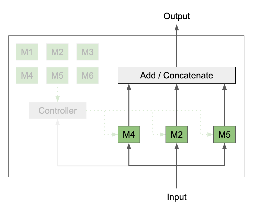
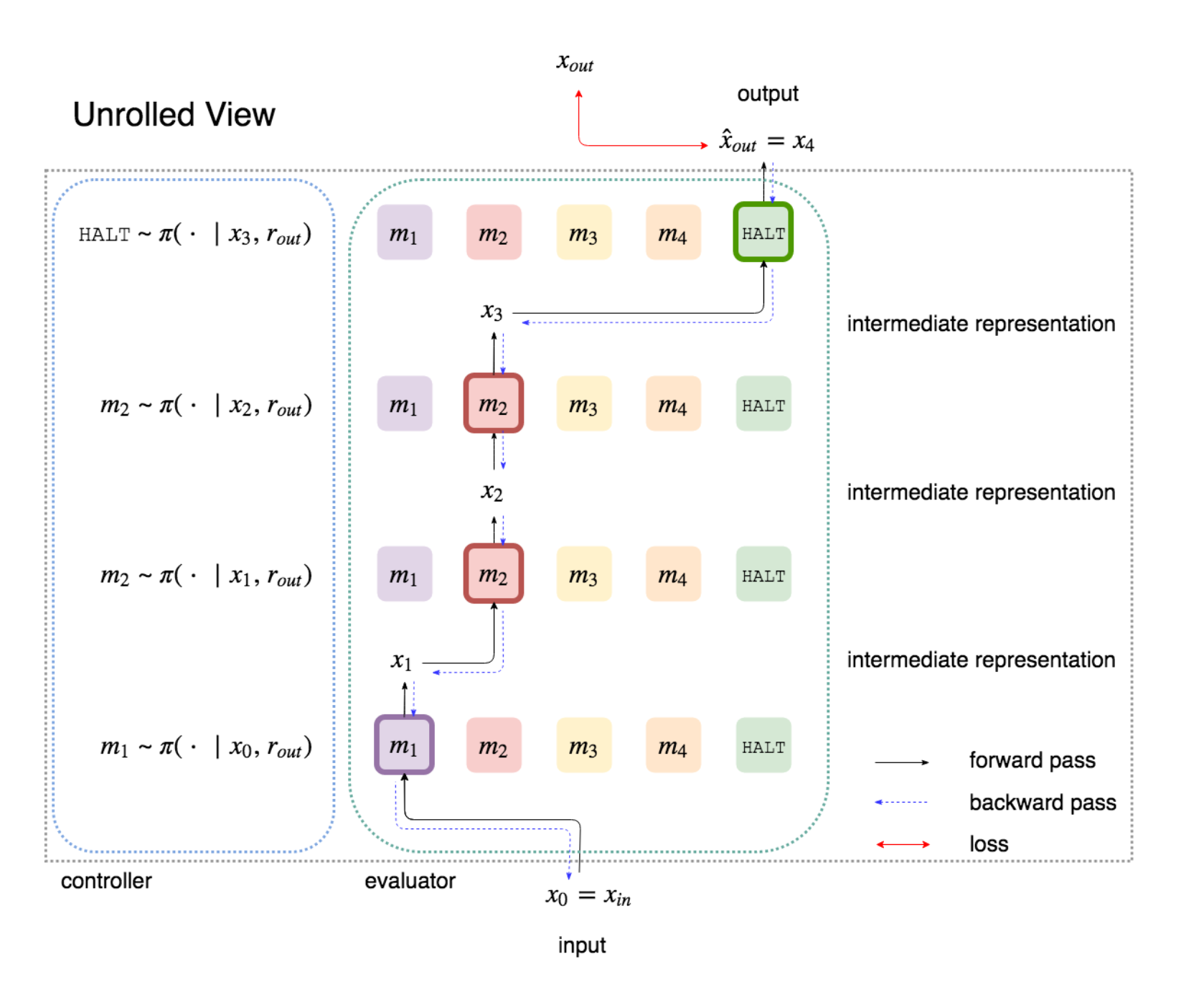
Pictorial examples of modular neural networks:
Why?
Why have modular neural architectures? Is it beneficial for program synthesis? Is it beneficial for machine learning in general?
Data invariances
Modularity Matters: Learning Invariant Relational Reasoning Tasks (Jo et al.)
When a dataset has a large number of invariances, a machine learning model must learn to associate a large number of seemingly unrelated patterns with one another, which may exacerbate the interference problem … One natural way to combat the interference problem is to allow for specialized sub-modules in our architecture. Once we modularize, we reduce the amount of interference that can occur between features in our model. These specialized modules can now learn highly discriminative yet invariant representations while not interfering with each other.
Strong generalization
Strong generalization means getting the right answer for an input/task that is very different from the training regime. Sometimes this is called zero-shot learning. Humans seem to be able to this. How does it work?
Learning Modular Neural Network Policies for Multi-Task and Multi-Robot Transfer (Devin et al.)
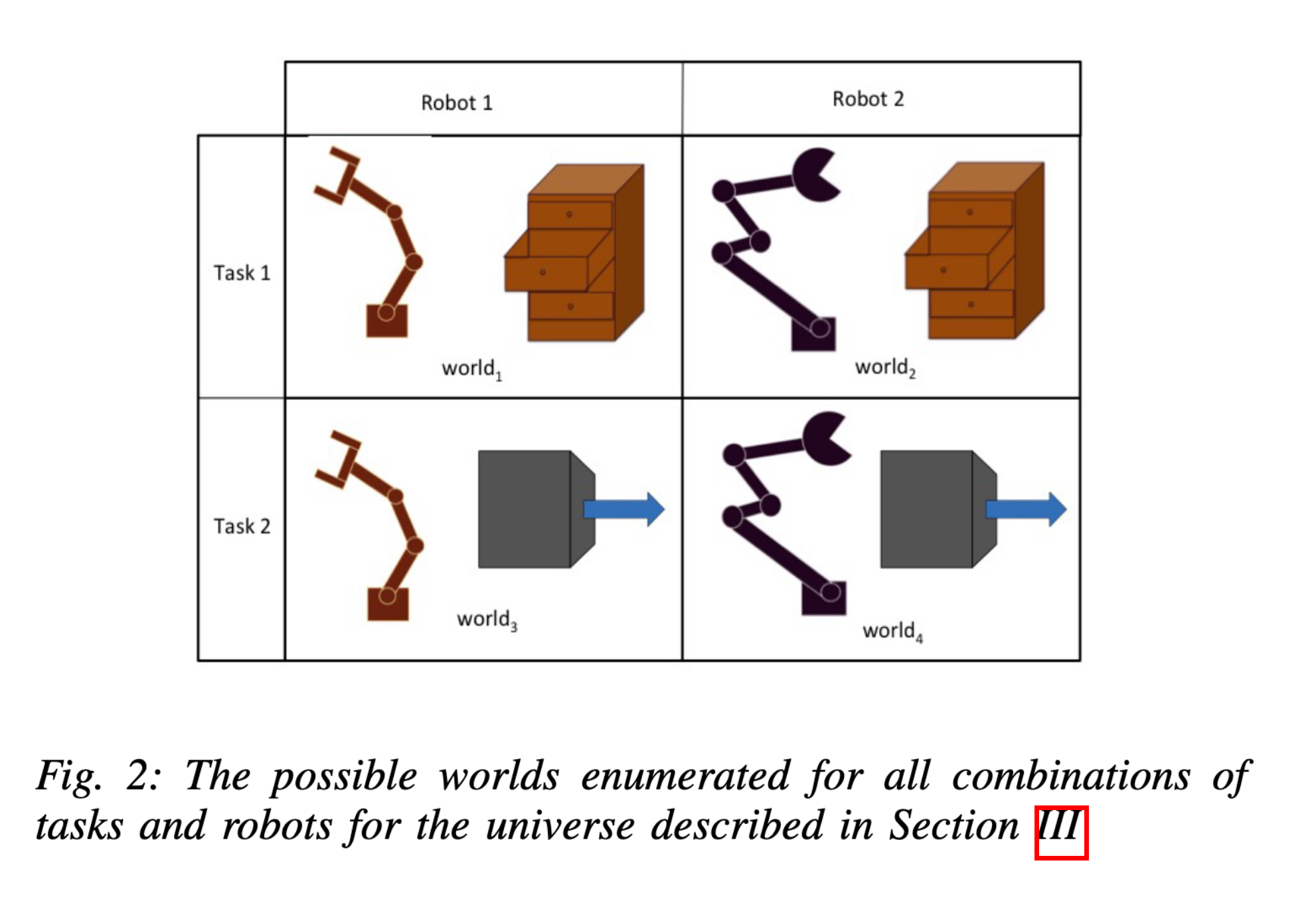
The robot and task networks are trained end-to-end on different robot-task combinations, with some held out. For example, during training this system does not encounter robot 2 combined with task 2, but does encounter robot 2 and task 2 separately in different situations. At test time, the system has to perform well when robot 2 is combined with task 2.
Modular Multitask Reinforcement Learning with Policy Sketches (Andreas 2016)
The modular structure of our approach, which associates every high-level action symbol with a discrete subpolicy,naturally induces a library of interpretable policy fragments that are easily recombined. This makes it possible to evaluate our approach under a variety of different data conditions: (1) learning the full collection of tasks jointly via reinforcement, (2) in a zero-shot setting where a policy sketch is available for a held-out task, and (3) in a adaptation setting, where sketches are hidden and the agent must learn to adapt a pretrained policy to reuse high-level actions in a new task.
… we have shown that it is possible to build agents that share behavior across tasks in order to achieve success in tasks with sparse and delayed rewards. This process induces an inventory of reusable and interpretable subpolicies which can be employed for zero-shot generalization when further sketches are available, and hierarchical reinforcement learning when they are not.
Parameter sharing
Convolutional and recurrent layers can be viewed as modular, in that they “stamp” a small neural network (with the same parameters) repeatedly in some pattern - repeated over space for CNNs, and repeated over time for RNNs.
Causal learning
Recurrent Independent Mechanisms (Goyal et al.)
Physical processes in the world often have a modular structure which human cognition appears toexploit, with complexity emerging through combinations of simpler subsystems. Machine learningseeks to uncover and use regularities in the physical world. Although these regularities manifestthemselves as statistical dependencies, they are ultimately due to dynamic processes governed bycausal physical phenomena.
The notion of independent or autonomous mechanisms has been influential in the field of causal inference. A complex generative model, temporal or not, can be thought of as the composition of independent mechanisms or “causal” modules. In the causality community, this is often considered a prerequisite for being able to perform localized interventions upon variables determined by such models (Pearl, 2009). It has been argued that the individual modules tend to remain robust or invariant even as other modules change, e.g., in the case of distribution shift (Schölkopf et al., 2012; Peterset al., 2017). This independence is not between the random variables being processed but between the description or parametrization of the mechanisms: learning about one should not tell us anything about another, and adapting one should not require also adapting another. One may hypothesize that if a brain is able to solve multiple problems beyond a single i.i.d. (independent and identically distributed) task, they may exploit the existence of this kind of structure by learning independent mechanisms that can flexibly be reused, composed and re-purposed.
An excerpt from Judea Pearl’s book Causality, 2nd ed.. Pearl refers to “mechanisms” as the nodes in a Bayesian network (e.g. depicted in figure 1.2), which are assumed to be modular: i.e. they are internally isolated, apart from causation traveling along their arrows, and they are reusable in the sense that the graph can be modified, which Pearl calls an intervention.
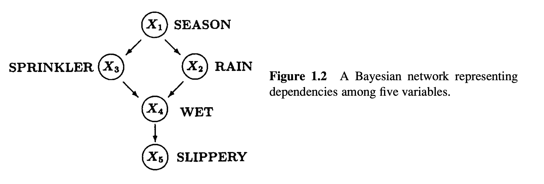
The example reveals a stronger sense in which causal relationships are more stable than the corresponding probabilistic relationships, a sense that goes beyond their basic ontological–epistemological difference. The relationship, “Turning the sprinkler on would not affect the rain,” will remain invariant to changes in the mechanism that regulates how seasons affect sprinklers. In fact, it remains invariant to changes in all mechanisms shown in this causal graph. We thus see that causal relationships exhibit greater robustness to ontological changes as well; they are sensitive to a smaller set of mechanisms. More specifically, and in marked contrast to probabilistic relationships, causal relationships remain invariant to changes in the mechanism that governs the causal variables ($X_3$ in our example).
Regardless of what use is eventually made of our “understanding” of things, we surely would prefer an understanding in terms of durable relationships, transportable across situations, over those based on transitory relationships. The sense of “comprehensibility” that accompanies an adequate explanation is a natural by-product of the transportability of (and hence of our familiarity with) the causal relationships used in the explanation. It is for reasons of stability that we regard the falling barometer as predicting but not explaining the rain; those predictions are not transportable to situations where the pressure surrounding the barometer is controlled by artificial means. True understanding enables predictions in such novel situations, where some mechanisms change and others are added. It thus seems reasonable to suggest that, in the final analysis, the explanatory account of causation is merely a variant of the manipulative account, albeit one where interventions are dormant. Accordingly, we may as well view our unsatiated quest for understanding “how data is generated” or “how things work” as a quest for acquiring the ability to make predictions under a wider range of circumstances, including circumstances in which things are taken apart, reconfigured, or undergo spontaneous change.
Program induction and synthesis
HOUDINI: Lifelong Learning as Program Synthesis (Valkov et al.)
In contrast to standard methods for transfer learning in deep networks, which re-use the first few layers of the network, neural libraries have the potential to enable reuse of higher, more abstract levels of the network, in what could be called high-level transfer.
… our results indicate that the modular representation used in HOUDINI allows it to transfer high-level concepts and avoid negative transfer. We demonstrate that HOUDINI offers greater transfer than progressive neural networks and traditional “low-level” transfer, in which early network layers are inherited from previous tasks.
Towards modular and programmable architecture search (Negrinho et al.)
The building blocks of our search spaces are modules and hyper-parameters. Search spaces are created through the composition of modules and their interactions.Implementing a new module only requires dealing with aspects local to the module. Modules and hyperparameters can be reused across search spaces, and new search spaces can be written by combining existing search spaces.
How?
How can modularity be achieved? Two things need to be simultaneously learned:
- The modules themselves.
- How the modules are to be connected together.
Key ideas:
- Routing: How the modules are connected together.
- Dynamic vs static routing: Static routing is fixed for all inputs, while dynamic routing is conditioned on a given input or context. A router is a function that outputs module routing given context.
- Soft vs hard routing: Soft routing is a weighted sum across all choices, while hard routing is a single discrete choice. Soft routing is differentiable while hard routing is not.
Examples of soft routing:
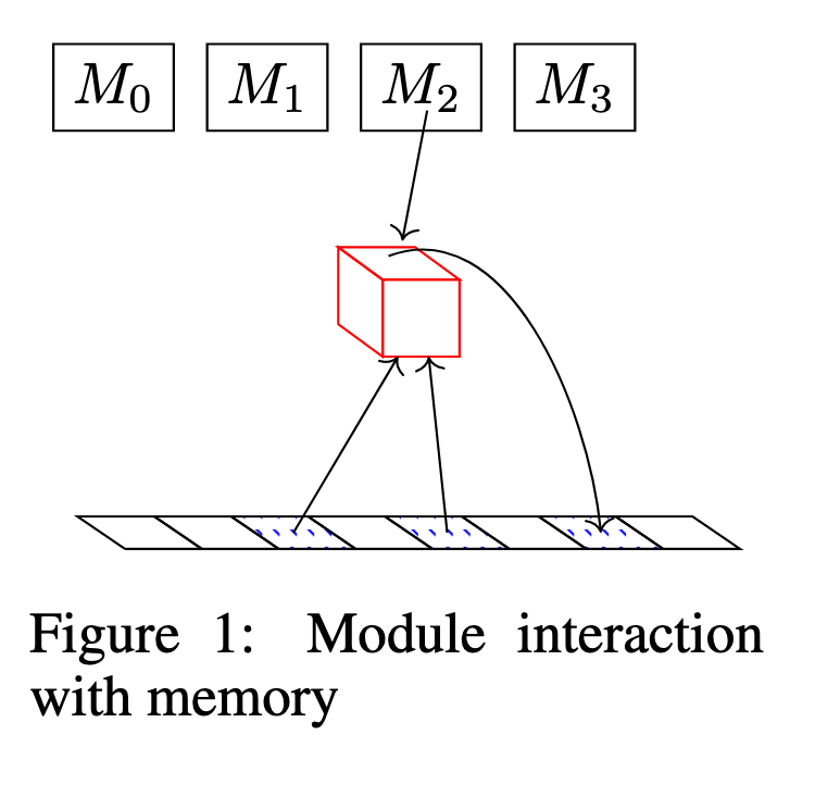
- Neural Turing Machines (Graves et al.)
- Differentiable neural computers (Graves et al.)
- Neural GPUs Learn Algorithms (Kaiser et al.)
Examples of hard routing:
- Automatically Composing Representation Transformations as a Means for Generalization (Chang et al.)
- Neural Random-Access Machines (Kurach et al.)
- Learning Simple Algorithms from Examples (Zaremba et al.)
Is there something in between soft and hard routing?
- Outrageously Large Neural Networks: The Sparsely-Gated Mixture-of-Experts Layer (Shazeer et al.)
- Modular Networks: Learning to Decompose Neural Computation (Kirsch et al.)
Module routing in detail
Following the setup in Kirsch et al.…
In the case of soft routing, think of module weights as probabilities. Instead of summing module outputs, sum probabilities of each possible output. This leads to a natural correspondence between soft and hard routing, where hard routing is sampled from the probability distribution.
In Kirsch et al., the choices are organized into layers, where for each layer $l$ a subset of $M$ modules are selected and their outputs are summed. In Abolafia et al., modules are connected into arbitrary computation graphs.
To keep things general, let $\mc{A}$ be a set of possible module routing choices, so that an element $a\in\mc{A}$ consists of all choices needed for the architecture to produce an output (e.g. which modules to use in the computation graph and how they are connected).
Given a routing choice $a\in\mc{A}$, the architecture output probability given input $x$ and parameters $\t$ is
$$
p(y\mid x,a,\t)\,.
$$
Under the hood this output probability may be arrived at by combining the following components:
- A collection of differentiable functions (modules) $f_{\t\up{i}}\up{i} : \mc{Z}\up{i} \to \mc{Z}\up{j}$ where $\mc{Z}\up{i}$ and $\mc{Z}\up{j}$ are latent spaces (e.g. vectors in $\R^n$), and $\t\up{i}$ are the function parameters. Typically $\t = (\t\up{1},\t\up{2},\dots)$ and each module has independent and isolated parameters. The input $x$ may be initially encoded into a latent space, or some modules may have $\mc{Z} = \mc{X}$ and the data can be fed in directly.
- A function $g$ that takes routing specification $a$, modules $\set{f_i}$, and input $x$, and outputs hidden representation $h$ (also a real vector).
- A distribution “head” on output space $\mc{Y}$, s.t. $h$ represents the parameters of the distribution. For example, a Gaussian $\mc{N}(y \mid h)$ where $h$ encodes a vector of means and a covariance matrix.
Putting these three things together produces the probability distribution $p(y\mid x,a,\t)$. Given training target $y$, this probability is fully differentiable w.r.t. $\t$ (typically given by the architecture as a logit, or log-probability). If routing choice $a$ were held fixed, we can train this architecture with standard supervised techniques, e.g. with SGD. Furthermore, if $a\up{k}$ can be provided by some external hard-coded system given training example $(x\up{k}, y\up{k})$, then we can use SGD to maximize the dataset log-probability
$$
\sum_{k=1}^N \log p(y\up{k}\mid x\up{k},a\up{k},\t)\,.
$$
This is essentially the used in Chang et al. and Andreas et al..
Ideally, we’d like to learn the module routing $a\up{k}$ for each training example $(x\up{k}, y\up{k})$. That means learning a routing function, which produces a routing $a\up{k}$ given input $x\up{k}$. Assuming $\mc{A}$ is a discrete space (routing choices are discrete, e.g. which modules to pick and how to connect them), we cannot differentiate such a function. RL could be used, as in Abolafia et al., but Kirsch et al. provides a more general perspective that allows for differentiation in principle, though intractable in practice.
Let the routing function output a probability distribution over $a\in\mc{A}$:
$$
p(a \mid x, \p)
$$
This router is comprised of a function $r_\p$, parameterized by parameters $\p$, that takes in $x$ and outputs a hidden representation $h'$ that, like before, holds the parameters for some probability distribution on $\mc{A}$ (e.g. Gaussian). If $a$ decomposes into a set of independent routing choices, e.g. $a=(a_1, a_2, \dots)$, then $p(a \mid x, \p) = \prod_t p(a_t \mid z_t, \p)$ where $\set{z_t}$ are potentially intermediate outputs from various modules, and at least one $z_t$ equals $x$.
This gives us a joint distribution on $y$ and $a$:
$$
p(y, a \mid x,\t,\p) = p(y\mid x,a,\t)p(a\mid x, \p)\,.
$$
To find the probability of $y$ given $x$, independent of routing choice $a$, we marginalize out $a$:
$$
p(y \mid x, \t, \p) = \sum_{a\in\mc{A}} p(y\mid x,a,\t)p(a\mid x, \p)\,.
$$
What this means in terms of training, is that if we are using naive SGD to maximize $\log p(y \mid x, \t, \p)$ w.r.t $\t$ and $\p$ jointly, then we simply sum over all possible routing choices in $\mc{A}$. In practice, this summation is intractable, since the number of routing decisions explodes as the number of modules is increased (as well as with other complexities like multi-input and multi-output modules).
We can view the same optimization through the lense of the REINFORCE algorithm, which naturally leads to RL optimization, where $p(a\mid x, \p)$ is the policy, $a$ are actions, and $x$ are environment observations. The reward function is then $R(a\mid x) = p(y\mid x,a,\t)$ (or the log-probability of $y$ like in Kirsch et al.). Let the loss function $\mc{L} = p(y \mid x, \t, \p)$. Then the gradient $\nabla_\p \mc{L}$ is given using the “log-trick”:
$$
\begin{aligned}
\nabla_\p \mc{L} &= \nabla_\p\E_{p(a\mid x, \p)}[p(y\mid x,a,\t)] \\
&= \nabla_\p\E_{p(a\mid x, \p)}[R(a \mid x)] \\
&= \E_{p(a\mid x, \p)}[\nabla_\p\log p(a\mid x, \p) R(a \mid x)]\,,
\end{aligned}
$$
which is the gradient as given in REINFORCE.
For the experiments in Abolafia et al., I found that scaling up episode collection as much as possible using IMPALA partially overcame the usual issues associated with RL: sparse reward, high variance gradients, and lack of stability. Stability is especially an issue when the modules are being trained at the same time, so that the reward being optimized is a moving target. We were not able to jointly learn module and routing, so in Abolafia et al. we settled for hard coded modules and focused on getting the router to work.
Other kinds of training
Kirsch et al. introduces a modified EM algorithm for simultaneously training $\t$ and $\p$, where routing choice $a$ is the latent variable. As with EM, this is a two step iterative process, where joint probability of $a$ and $x$ is maximized with fixed $a$, and then $a$ is locally improved according to the current probability distribution. Rather than finding the argmax $a$, which is intractable, Kirsch et al. samples an i.i.d. batch from $p(a \mid x, \p)$ and updates $a$ only if a higher probability $a$ is found.
This training algorithm can be viewed as performing policy gradient training (RL) with a “top-$K$” buffer, as described in Neural Program Synthesis with Priority Queue Training (Abolafia 2018), where $K=1$.
Here is the general case of this training procedure:
Let $\tilde{A}_n$ be a length-$S$ i.i.d. sample from $p(a_n \mid x_n,\p)$.
Let $A_n^*$ be a top-$K$ buffer for the $n$-th training example $(x\up{n},y\up{n})$. That means $A_n^*$ holds the best $a_n$ observed over the course of training, scored by $p(a_n \mid x_n,\p)$. Note that this is a moving target, since $\p$ is simultaneously changing, so the joint score of $A_n^*$ can decrease.
Let $A_n = \tilde{A}_n \cup A_n^*$.
Let $B \subseteq D$ be a minibatch. The Monte Carlo gradient approximation (ala REINFORCE) is:
$$
\nabla_\p\mc{L} \approx \frac{1}{\abs{B}}\sum_{n\in B}\frac{1}{\abs{A_n}}\sum_{a_n \in A_n} \nabla_\p\log p(a\mid x, \p) R(a \mid x)
$$
where $R(a\mid x) = p(y\mid x,a,\t)$ or $\log p(y\mid x,a,\t)$.
If $A_n^* = \emptyset$ this setup reduces to usual policy gradient training, and if $\tilde{A}_n = \emptyset$ and $\abs{A_n^*}=1$ (i.e. $K=1$) this reduces to the EM algorithm (Algorithm 1) in Kirsch et al..
Abolafia 2018 is similar (where $K\geq 1$), except that the reward function is assumed to be fixed through out training, so the top-$K$ buffer $A_n^*$ cannot diminish in total score over time.
Information theory
Kirsch et al. plots the quantities $H_a$ and $H_b$ as diagnostic tools and measures of “module collapse” and training convergence. I used the same quantities in my own experiments and found them to be similarly helpful.
There is theoretical justification for these quantities, and they may even be used as regularizers.
Let $A$ be the routing random variable and let $X$ be the input random variable, distributed jointly by $p(a \mid x, \p)p(x)$ where $p(x)$ is the true and unknown input distribution.
The mutual information between $A$ and $X$ decomposes:
$$
\I(A, X) = \H(A) - \H(A \mid X)
$$
We cannot explicitly compute these entropy terms because we do not have access to $p(x)$ or $p(a \mid \p)$.
Assume we can only explicitly compute $p(a \mid x, \p)$. Let’s also suppose that we can explcitily compute $\H(A \mid X=x) = -\sum_{a\in\mc{A}} p(a \mid x, \p) \log p(a \mid x, \p)$. Though summing over $\mc{A}$ is still intractable, if we suppose that the routing distribution factors into independent choices which are themselves tractable to enumerate (like the choice for each layer in Kirsch et al.): $\mc{A} = \mc{A}_1\times\mc{A}_2\times\dots$ and $a = (a_1, a_2, \dots) \in \mc{A}$ s.t.
$$
p(a \mid x, \p) = \prod_{l=1}^L p(a_l \mid x, \p_l)\,,
$$
then we can tractably compute the conditional entropy as the sum of entropies of each choice:
$$
\begin{aligned}
\H(A \mid X=x) &= \sum_{l=1}^L \H(A_l \mid X=x) \\
&= \sum_{l=1}^L \sum_{a_l\in\mc{A}_l} p(a_l \mid x, \p_l) \log p(a_l \mid x, \p_l)\,.
\end{aligned}
$$
Now we can do a Monte Carlo approximation of the entropy terms of interest using the existing dataset. The statistical properties of this MC estimation is discussed in On Variational Bounds of Mutual Information. Let $B \subseteq D$ be a minibatch uniformly sampled from dataset $D$.
$$
\begin{aligned}
\H(A \mid X) &= -\E_{p(x)}[\H(Y\mid X=x)] \\
&\approx \frac{1}{\abs{B}}\sum_{n \in B} \H(Y\mid X=x_n)
\end{aligned}
$$
Letting $q(a \mid \p)$ be a Monte Carlo approximation of the marginal distribution $p(a\mid \p)$, derived from
$$
\begin{aligned}
p(a \mid \p) &= \E_{p(x)}p(a \mid x, \p) \\ &\approx \frac{1}{\abs{B}}\sum_{n \in B}p(a \mid x, \p) \\
&= q(a\mid \p)\,,
\end{aligned}
$$
we can approximate the marginal entropy,
$$
\begin{aligned}
\H(A) &= -\E_{p(a \mid \p)}[\log p(a \mid \p)] \\
&\approx -\E_{q(a \mid \p)}[\log q(a\mid \p)]\,.
\end{aligned}
$$
We can think of $\I$ as measuring the bijectivness of the mapping from $x$ to $a$, where $\H(A)$ measures surjectivity and $\H(A\mid X)$ measures anti-injectivity. See http://zhat.io/articles/primer-shannon-information#expected-mutual-information.
$\H(A)$ measures module use. If its maximized, all the modules are getting used equally often.
$\H(A\mid X)$ measures convergence. If its maximized, then the router is completely confident that there is exactly one appropriate routing choice for any given input.
The ideal is that all modules get used often and the router thinks there is one routing choice per input.
$\H(A)$ is a typical RL regularizer (called entropy regularization, see A3C). However maximizing $\I(A,X)$ (where $x$ are env states) is uncommon. It may be unnecessary since $p(a \mid x)$ naturally becomes peaky over the course of training.