[This is an article, which is something I’ve optimized for readability and transmission of ideas, opposed to notes that are the seed of an idea and something I’ve written quickly.]

The definition of causality within physics is not a settled matter, perhaps surprisingly. My understanding is that this question is studied more by philosophers than physicists, as the field of physics tends to avoid interpretational problems. That is to say, theories like relativity or quantum mechanics are mathematically well defined and make predictions, so that’s all there is to it, right? I’m not a physicist, so I will proceed to ask such questions.

I suspect that causality and information are intimately related. To initiate my pursuit to understand physical information, I am starting by trying to understand the role causality plays in physics. The SEP outlines some of the conversation and ideas around causality and physics. I haven’t read these ideas yet, but I want to take my own tabula rasa stab at the problem before reading about what other people have tried. I am familiar with Judea Pearl’s notion of causality in machine learning and statistics, which I will attempt to apply to physics below.

Causal Models

First, I’ll outline Pearl’s framework for causality. I used Causality (Pearl) and Elements of Causal Inference (Peters, Janzing, Schölkopf) to learn about this topic.

Pearl assumes the world (or some part of it) can be represented by graph, where nodes represent potential observations, and their directed edges represent causal links. For example (from Pearl):

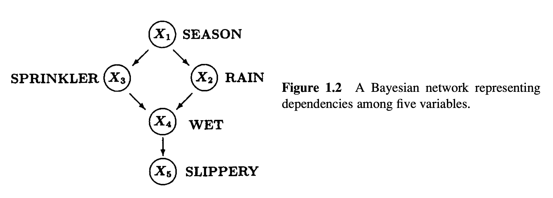
The core idea in Pearl’s causality is the intervention, which is a modification to the graph where a node is disconnected from all incoming arrows and held fixed at some value.

An example of an intervention:

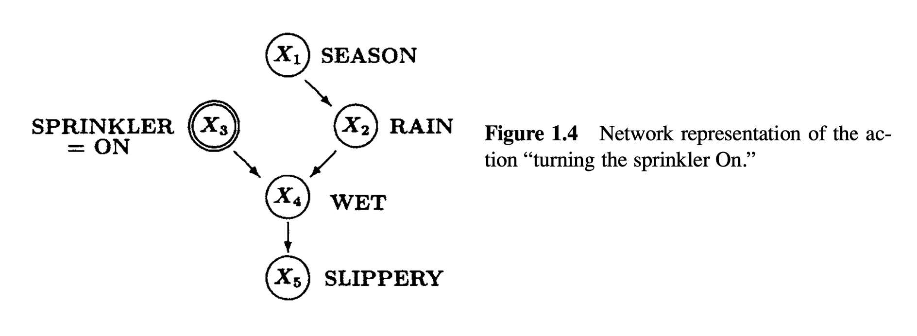
An intervention in this graph is a graph surgery (as Pearl calls it). Graph interventions correspond to real-world interventions. The intervention depicted above corresponds to someone forcing the sprinkler system to turn on (e.g. by switching the sprinkler system’s setting from auto to manual). The sprinkler state is now causally independent of everything else in the graph, because we, the experimenters, have directly determined its state (we would need to be careful to ensure our own actions are not causally linked to the system we are studying). By observing the down stream effects of this change to the graph, the causal effect of the particular node $X_3$ can be measured. That is the effect of $X_3$, independent of other nodes like $X_1$.

Generally Pearl places a probability distribution on graph node states, given by $P(X_1=x_1,X_2=x_2,X_3=x_3,\dots )$, or using shorthand, $P(x_1,x_2,x_3,\dots )$. I’ll use capital letters, $X_i$, to denote graph nodes themselves (or random variables on graph nodes), and lowercase letters, $x_i$, to denote a specific value that the correspond node takes on. So for example, node $X_3$, the sprinkler state, could take on the values $\mathrm{ON}$ or $\mathrm{OFF}$. In the abstract, $X_3$ takes on some value $x_3$. Sometimes I’ll introduce a “prime” tick, $x_3^{\prime }$, to denote some other value that may be distinct from $x_3$.

There is an alternative functional perspective, where each node’s value is a deterministic function of incoming values traveling along inward arrows, and an auxiliary noise input not depicted in the graph. Those noise inputs can themselves be determined (i.e. held fixed), but be pulled from an algorithmically random stream. I will stick to the deterministic perspective when I discuss physics, while recognizing that random physical processes can be viewed as deterministic but algorithmically random.

Quoting Causality, section 1.4.1, Structural Equations:

In its general form, a functional causal model consists of a set of equations of the form
$$x_i=f_i(p{a}_i,u_i),i=1,\dots ,n,$$
where $p{a}_i$ (connoting parents) stands for the set of variables that directly determine the value of $X_i$ and where the $U_i$ represent errors (or “disturbances”) due to omitted factors.

That is to say, the parents $P{A}_i$ of node $X_i$ is the set of nodes with arrows pointing into $X_i$. So in the example, $P{A}_3=\left\{X_1\right\}$ because $X_1$ is the only node pointing into $X_3$, and $P{A}_4=\{X_2,X_3\}$ because both $X_2$ and $X_3$ point into $X_4$. Node $X_1$ is not a direct parent of $X_4$.

$U_i$ is an auxiliary input node to each $X_i$ which is not depicted in the graph, which makes the output value $x_i$ random. In my view, each value $u_i$ is pulled from an algorithmically random stream. Given the set of values $p{a}_i$ and value $u_i$, the output of the function $f_i$ is then able to be random.

A note about notation: It would not be correct to write $f_i(P{A}_i,U_i)$ which passes the nodes themselves into the function $f_i$. On the other hand, $f_i(p{a}_i,u_i)$ is passing the values $p{a}_i$ of the parent nodes $P{A}_i$ and $u_i$ of the noise input node $U_i$ into the function.

Do-Operator

If $P$ is the probability measure on the initial graph (e.g. figure 1.2 above), then what is the probability measure on the modified graph after taking an intervention (e.g. figure 1.4)? Pearl uses “do”-notation, which for the example above looks like this:

$$P(x_1,x_2,x_3,x_4,x_5\mid \mathrm{do}(X_3=\mathrm{ON})).$$

This is the probability of the vector of node values $(x_1,x_2,x_3,x_4,x_5)$ given that the intervention setting node $X_3$ to constant value $\mathrm{ON}$ was taken. Note the notational similarity to conditional probability: $P(x_1,x_2,x_3,x_4,x_5\mid X_3=\mathrm{ON})$. Conditionalization is a different operation on the measure $P$ than the “do”-operator, but they are mathematically related and their similar notation is justified.

For an arbitrary graph with nodes $X_1,\dots ,X_n$, and probability measure $P$ on node values, the conditional probability of value vector $(x_1,\dots ,x_n)$ given $X_i=x_i^{\prime }$ is

$$P(x_1,\dots ,x_n\mid x_i^{\prime })=\{\begin{array}{ll}\frac{P(x_1,\dots ,x_n)}{P(x_i^{\prime })}& x_i=x_i^{\prime }\\ 0& x_i\ne x_i^{\prime }\end{array}$$

whereas the probability of $(x_1,\dots ,x_n)$ given that intervention $\mathrm{do}(X_i=x_i^{\prime })$ was taken is (Causality, eq 3.11)

$$P(x_1,\dots ,x_n\mid \mathrm{do}(x_i^{\prime }))=\{\begin{array}{ll}\frac{P(x_1,\dots ,x_n)}{P(x_i^{\prime }\mid p{a}_i)}& x_i=x_i^{\prime }\\ 0& x_i\ne x_i^{\prime }\end{array}$$

Both operations are performing a domain restriction on $P$, in the sense that the resulting measure assigns 0 probability to all vectors $(x_1,\dots ,x_n)$ where $x_i\ne x_i^{\prime }$, for some constant $x_i^{\prime }$. The difference between them is that conditionalization, $P(x_1,\dots ,x_n\mid x_i^{\prime })$, simply rescales the resulting measure by $1/P(x_i^{\prime })$ after domain restriction, whereas intervention, $P(x_1,\dots ,x_n\mid \mathrm{do}(x_i^{\prime }))$, re-weights every single probability independently by $1/P(x_i^{\prime }\mid p{a}_i)$, where $p{a}_i$ is the set of values in $(x_1,\dots ,x_n)$ for the parent nodes $P{A}_i$ of node $X_i$.

Rewriting $P(x_1,\dots ,x_n)$, we can see why multiplying by $1/P(x_i^{\prime }\mid p{a}_i)$ corresponds to an intervention:

$$P(x_1,\dots ,x_n)=\prod _{j=1}^{n}P(x_j\mid p{a}_j),$$

by the chain rule of probability, because the graph also encodes which nodes are statistically independent, i.e. if $x_k\notin p{a}_j$, then $P(x_j\mid x_k)=P(x_j)$.

The operation of removing the connections going into $X_i$ from the parents $P{A}_i$ is a matter of removing the term $P(x_i\mid p{a}_i)$ by dividing it out.

This formulation of an intervention can be generalized further. Instead of setting $X_i$ to a constant value $x_i^{\prime }$, in general, we can replace the node distribution $P(X_i\mid P{A}_i)$ with the new distribution $Q(X_i\mid P{A}_i^{\prime })$ where $P{A}_i^{\prime }$ is some new set of parents, which may or may not be the empty set, or equivalent to or overlap with the old parents $P{A}_i$. If $P{A}_i^{\prime }$ is empty, that is equivalent to making $Q$ statistically independent where $Q(X_i\mid P{A}_i)=Q(X_i)$. We can get our constant-value intervention by choosing a delta distribution (one-hot for discrete $X_i$, and Dirac delta for continuous $X_i$) $Q(X_i)={\delta }_{x_i^{\prime }}$ which is non-zero only if $X_i=x_i^{\prime }$. Now this general-case intervention is replacing the term $P(X_i\mid P{A}_i)$ with $Q(X_i\mid P{A}_i^{\prime })$, which looks like this:

$$\begin{array}{rl}& P(x_1,\dots ,x_n|\mathrm{do}\{P(x_i\mid p{a}_i)\to Q(x_i\mid p{a}_i^{\prime })\})\\ \\ & =P(x_1,\dots ,x_n)\frac{Q(x_i\mid p{a}_i^{\prime })}{P(x_i\mid p{a}_i)}.\end{array}$$

When $Q(x_i\mid p{a}_i^{\prime })=Q(x_i)={\delta }_{x_i^{\prime }}$ this expression reduces to the constant-value intervention defined above.

In the functional perspective, an intervention replaces $f_i(p{a}_i,u_i)$ with some other function $f_i^{\prime }(p{a}_i^{\prime },u_i)$.

Causal Effect

In Causality, definition 3.2.1, Pearl defines causal effect as follows:

Let $X$ and $Y$ be two disjoint sets of graph nodes. The causal effect of $X$ on $Y$ is the function $\mathcal{E}$ from the space of node values for $X$ to the space of probability measures on $Y$,

$$\mathcal{E}(x)=P(Y\mid \mathrm{do}(X=x)),$$

where $x$ is some chosen vector of values for the nodes $X$.

That is to say, the causal effect of nodes $X$ on nodes $Y$ is characterized by the set of all interventions obtained setting $X$ to every possible value $x$, where each intervention is characterized by a change in probability distribution on $Y$. That is to say, the causal effect of $X$ on $Y$ is characterized by how $P(Y\mid \mathrm{do}(X=x))$ varies for different $x$, and compared to no intervention $P(Y)$.

When Interventions And Conditionalization Are Equivalent

It should be obvious that when node $X_i$ has no parents then $P(x_{1:n}\mid \mathrm{do}(x_i^{\prime }))=P(x_{1:n}\mid x_i^{\prime })$ for all node values $x_i^{\prime }$, because $P{A}_i=\mathrm{\varnothing }$ and so $P(x_i^{\prime }\mid p{a}_i)=P(x_i^{\prime })$.

Another case is when we are only considering the marginal distribution on a subset of variables. Then the conditional distribution and intervention distribution on the Markov blanket of that subset are equivalent.

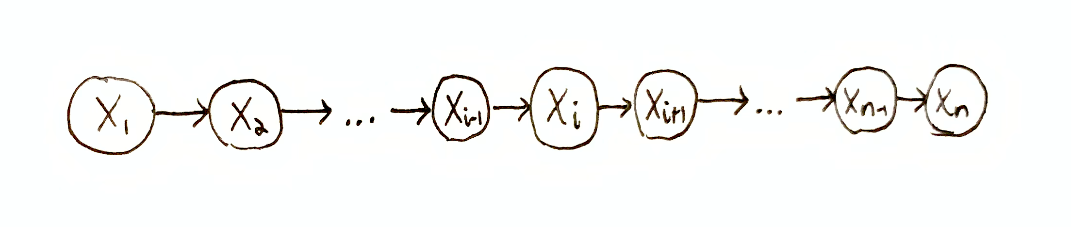
To see what I mean, let’s consider the Markov chain $X_1,\dots ,X_n$ where $P(x_1,\dots ,x_n)=P(x_n\mid x_{n-1})P(x_{n-1}\mid x_{n-2})\dots P(x_2\mid x_1)P(x_1)$ and $P{A}_i=\left\{X_{i-1}\right\}$ for all $i>1$. Then we have

$$\begin{array}{rl}& P(x_n,\dots ,x_{i+1}\mid \mathrm{do}(x_i^{\prime }))\\ & =\sum _{x_{i-1},\dots ,x_1}P(x_n,\dots ,x_1\mid \mathrm{do}(x_i^{\prime }))\\ & =\{\begin{array}{ll}\sum _{x_{i-1},\dots ,x_1}\frac{P(x_n,\dots ,x_{i+1}\mid x_i)P(x_i\mid x_{i-1})P(x_{i-1},\dots ,x_1)}{P(x_i^{\prime }\mid x_{i-1})}& x_i=x_i^{\prime }\\ 0& x_i\ne x_i^{\prime }\end{array}\\ & =\sum _{x_{i-1},\dots ,x_1}P(x_n,\dots ,x_{i+1}\mid x_i^{\prime })P(x_{i-1},\dots ,x_1)\\ & =P(x_n,\dots ,x_{i+1}\mid x_i^{\prime }).\end{array}$$

Causality For Physics

Pearl’s causality is based on the idea of the intervention, which is a kind of graph surgery.

To apply Pearl’s causality to physics, we’d need to define what an intervention does to physical processes. There are two immediate problems:

1. Pearl defines interventions for causal graphs, where node values are sampled i.i.d., and the nodes represent are stateless and otherwise isolated processes (aside from their arrows). Physics, on the other hand, allows for arbitrary interactions between systems, to the point where the boundaries between systems may be blurred or destroyed so that it does not even make sense to think about there being any independent components at all (think about a liquid or gas). Physical processes are not i.i.d. (the future depends on the past), and they have internal state which determines their future time evolution.
2. Classical physics is non-probabilistic (non-statistical Newtonian mechanics and relativity). If our notation of causality is to be suitable to all of physics, we need to apply to Newtonian mechanics, which means causality must precede probability. Therefore we need to define interventions on deterministic systems.

Pearl generally considers a graph intervention to represent an intervention that can conceivably be taken, and ideally taken recently so that the causal effect of various interventions can be empirically estimated with histograms (empirically estimate $P(Y\mid \mathrm{do}(X))$ and $P(Y)$).

I don’t think physical plausible interventions can generalize to arbitrary physical systems. I will instead consider what I call a counterfactual intervention, which is merely a modification to a mathematical model (i.e. representation) of physics. A counterfactual intervention is hypothetical, and produces a different time-line than the “factual” time-evolution of the system. A counterfactual intervention is the answer to the question, “what would have happened if the system were in state $x^{\prime }$ rather than state $x$ at time $t$?”

If intuition serves right and the logical structure of causality lies within all theories of physics, the purpose of the counterfactual intervention is to probe those theories to make their implicit causal structures mathematically explicit.

My objective here is to define an abstract definition for theories of physics in general, define what it means to take a counterfactual intervention on a physical system (both probabilistic or non-probabilistic), and then to show the equivalence of this type of intervention to Pearl’s graph intervention above.

Abstract Physics

In any theory of physics there is a state space $\mathrm{\Omega }$. In Newtonian mechanics, state is a vector of various components of the system, such as a vector of positions and momenta given by $\omega =(\overrightarrow{q},\overrightarrow{p})\in \mathrm{\Omega }$. In general state can include other kinds of degrees of freedom such as the orientation of solid bodies in 3D space. In quantum mechanics there is quantum state, and state spaces are Hilbert spaces.

A theory of physics specifies both the state space $\mathrm{\Omega }$ and how to solve for the time-evolution of the system given a particular state ${\omega }_t$ at time $t$. The result is a complete description of a system’s time evolution through state space given as a state-function of time, $\sigma :\mathbb{R}\to \mathrm{\Omega }:t\mapsto \sigma (t)$, which I’ll call a trajectory. To be clear, a single trajectory $\sigma$ is a single possible time-evolution, e.g. where $\sigma (t)={\omega }_t$.

The mathematical machinery that converts known information, e.g. the state of the system at time $t$, varies between theories of physics and often makes use of a Lagrangian or Hamiltonian. These details can be abstracted away. In principle, for any theory of physics there is a family of time-evolution functions ${\tau }_{\mathrm{\Delta }t}:\mathrm{\Omega }\to \mathrm{\Omega }$ (also called propagators), for every time interval $\mathrm{\Delta }t\in \mathbb{R}$ (both positive and negative) which maps any state $\omega \in \mathrm{\Omega }$ at time $t$ to the state at time $t+\mathrm{\Delta }t$. Typically physics is time-symmetric, which means that ${\tau }_{\mathrm{\Delta }t}$ is a bijection and thus invertible. Note also that ${\tau }_{\mathrm{\Delta }t}$ does not depend on the absolute time $t$, and so we are implicitly assuming the given theory of physics is time-translationally invariant.

The set of all trajectories is $\mathbb{R}\to \mathrm{\Omega }$, denoting the set of all functions from $\mathbb{R}$ to $\mathrm{\Omega }$. For a given time-evolution family $\tau$, there is a subset of trajectories which are valid for $\tau$ (or $\tau$-valid),

$$\mathrm{\Sigma }=\{\sigma :\mathbb{R}\to \mathrm{\Omega }\mid \mathrm{\forall }t,\mathrm{\Delta }t\in \mathbb{R}:\sigma (t+\mathrm{\Delta }t)={\tau }_{\mathrm{\Delta }t}(\sigma (t))\}.$$

Incorporating Probability

Suppose we want to work with some kind of statistical physics. Perhaps we are uncertain about which state the system is in, or the state is randomly chosen. We can just as easily put a probability measure on the set of trajectories.

Let $M$ be a probability measure on the set of all trajectories $\mathbb{R}\to \mathrm{\Omega }$. Moreover, we want to require $M$ to obey the physics of $\tau$ and assign zero probability to physically impossible trajectories, i.e. $\tau$-invalid trajectories. Specifically, $M$ should assign 0 probability to any set comprised only of $\tau$-invalid trajectories, or equivalently, $M(\mathrm{\Sigma })=1$ (if $M$ is a normalized measure).

This is not typically how statistical physics is conceived of. Normally, there is a probability measure on states at time $t$, and time evolution time-evolves that measure. Instead, I’ve put a static global measure $M$ on entire trajectories. However, these two views are equivalent.

Let ${\mu }_t$ be the marginal probability measure on state space $\mathrm{\Omega }$ of the “system” at time $t$. Specifically, ${\mu }_t$ is the unique marginal distribution of $M$ on time $t$ only, given by

$${\mu }_t(\mathcal{O})=M\{\sigma :\mathbb{R}\to \mathrm{\Omega }\mid \sigma (t)\in \mathcal{O}\},$$

for (measurable) state subsets $\mathcal{O}\subseteq \mathrm{\Omega }$. Then ${\mu }_{t+\mathrm{\Delta }t}$ is then the time-evolution of measure ${\mu }_t$, given by

$${\mu }_{t+\mathrm{\Delta }t}(\mathcal{O})={\mu }_t({\tau }_{\mathrm{\Delta }t}^{-1}(\mathcal{O})).$$

Proof that ${\mu }_t({\tau }_{\mathrm{\Delta }t}^{-1}(\mathcal{O}))=M\{\sigma :\mathbb{R}\to \mathrm{\Omega }\mid \sigma (t+\mathrm{\Delta }t)\in \mathcal{O}\}$:
$M\{\sigma :\mathbb{R}\to \mathrm{\Omega }\mid \sigma (t+\mathrm{\Delta }t)\in \mathcal{O}\}$
$=M\{\sigma \in \mathrm{\Sigma }\mid \sigma (t+\mathrm{\Delta }t)\in \mathcal{O}\}+M\{\sigma \in \bar{\mathrm{\Sigma }}\mid \sigma (t+\mathrm{\Delta }t)\in \mathcal{O}\}$
$=M\{\sigma \in \mathrm{\Sigma }\mid \sigma (t+\mathrm{\Delta }t)\in \mathcal{O}\}+0$.
$\{\sigma \in \mathrm{\Sigma }\mid \sigma (t+\mathrm{\Delta }t)\in \mathcal{O}\}=\{\sigma \in \mathrm{\Sigma }\mid \sigma (t)\in {\tau }_{\mathrm{\Delta }t}^{-1}(\mathcal{O})\}$ by the definition of $\mathrm{\Sigma }$.
$M\{\sigma \in \mathrm{\Sigma }\mid \sigma (t)\in {\tau }_{\mathrm{\Delta }t}^{-1}(\mathcal{O})\}$
$=M\{\sigma :\mathbb{R}\to \mathrm{\Omega }\mid \sigma (t)\in {\tau }_{\mathrm{\Delta }t}^{-1}(\mathcal{O})\}$
$={\mu }_t({\tau }_{\mathrm{\Delta }t}^{-1}(\mathcal{O}))$ by the definition of ${\mu }_t$. $◼$

Proof that $M$ is uniquely determined by ${\mu }_t$, so long as ${\tau }_{\mathrm{\Delta }t}$ is a bijection and $M(\mathrm{\Sigma })=1$.

At time $t$, for each $\omega \in \mathrm{\Omega }$, there is a unique $\tau$-valid trajectory $\sigma$ that passes through $\omega$, given by the mapping $t^{\prime }\mapsto {\tau }_{t^{\prime }-t}(\omega )$. Therefore, there is a family of bijections between the $\tau$-valid trajectories $\mathrm{\Sigma }$ and state space $\mathrm{\Omega }$:

$${\mathrm{\Gamma }}_t:\mathrm{\Omega }\to \mathrm{\Sigma }:\omega \mapsto (t^{\prime }\mapsto {\tau }_{t^{\prime }-t}(\omega )),$$

for all $t\in \mathbb{R}$. So ${\mathrm{\Gamma }}_t(\omega )=\sigma$ where $\sigma (t)=\omega$ and $\sigma$ is $\tau$-valid. The inverse is then ${\mathrm{\Gamma }}_t^{-1}(\sigma )=\sigma (t)$. I haven’t defined proper measure spaces on trajectories and states, so I will just assume ${\mathrm{\Gamma }}_t$ is a measurable function.

We can derive the following relation:
${\mu }_t(\mathcal{O})=M\{\sigma :\mathbb{R}\to \mathrm{\Omega }\mid \sigma (t)\in \mathcal{O}\}$
$=M\{\sigma \in \mathrm{\Sigma }\mid \sigma (t)\in \mathcal{O}\}$
$=M{\mathrm{\Gamma }}_t\mathcal{O}$.

Thus for any (measurable) subset of trajectories $S\subseteq (\mathbb{R}\to \mathrm{\Omega })$, there is a corresponding (measurable) subset of states $\mathcal{O}={\mathrm{\Gamma }}_t^{-1}(S\cap \mathrm{\Sigma })$ so that $M(S)=M(S\cap \mathrm{\Sigma })=M({\mathrm{\Gamma }}_t{\mathrm{\Gamma }}_t^{-1}(S\cap \mathrm{\Sigma }))=M({\mathrm{\Gamma }}_t\mathcal{O})={\mu }_t(\mathcal{O})$. $◼$

Interventions For Physics

Let $I:\mathrm{\Omega }\to \mathrm{\Omega }$ be a state-replacement function. Usually we want $I$ to be some kind of state projection function where $I(\mathrm{\Omega })\subset \mathrm{\Omega }$ is a strict subset.

I will define a “do”-operator on individual trajectories which performs a surgery and outputs a modified trajectory. Specifically, given state-replacement function $I$ and time $T$,

$$\underset{I⇝T}{\mathrm{do}}[\sigma ](t)\stackrel{\mathrm{def}}{=}\{\begin{array}{ll}\sigma (t)& t<T\\ {\tau }_{t-T}(I(\sigma (T)))& t\ge T\end{array}.$$

The resulting trajectory is identical to $\sigma$ prior to time $T$, and discontinuously jumps at time $T$ to the alternative $\tau$-valid trajectory starting from state $I(\sigma (T))$. In this way, $I$ determines which trajectory “tail” to attach to the given trajectory “head” $\sigma$. The resulting “Frankenstein”-trajectory is usually not globally $\tau$-valid, but its head and tail are guaranteed to be $\tau$-valid, and thus is locally $\tau$-valid everywhere except across time $T$.

Let’s overload this “do”-operator to apply element-wise to sets, so

$${\mathrm{\Sigma }}^{\prime }=\underset{I⇝T}{\mathrm{do}}\mathrm{\Sigma }=\{\underset{I⇝T}{\mathrm{do}}[\sigma ]|\sigma \in \mathrm{\Sigma }\}.$$

Starting with the measure $M$ from above, applying $\underset{I⇝T}{\mathrm{do}}$ to the set of all trajectories $\mathbb{R}\to \mathrm{\Omega }$ induces a transformed measure $M^{\prime }$, where for subsets $S^{\prime }\subseteq (\mathbb{R}\to \mathrm{\Omega })$,

$$M^{\prime }(S^{\prime })=M\left({\underset{I⇝T}{\mathrm{do}}}^{-1}{S}^{\prime }\right)=M\{\sigma \in \mathrm{\Sigma }|\underset{I⇝T}{\mathrm{do}}[\sigma ]\in S^{\prime }\}.$$

This conception of intervention is different from Pearl’s, which is a modification of the functions generating the behavior of the process in question. In my formulation, I am modifying the state of the process at some point in time, but keeping the behavior-generating-functions, i.e. $\tau$, unchanged. That is to say, I am modifying systems, but not the physics, whereas Pearl is modifying the physics, so to speak.

Proof of Pearl-Equivalence

The question is whether my definition of an intervention is equivalent with Pearl’s. To prove this, I need to put my intervention in terms of Pearl’s setup.

The measure $M$ on trajectories corresponds to the measure $P$ on graph states, and the transformed measure $M^{\prime }$ corresponds to the transformed measure $P(\dots \mid \mathrm{do}(\dots ))$ on the modified graph.

Recall that $M^{\prime }$ is defined by

$$M^{\prime }(S^{\prime })=M\{\sigma \in \mathrm{\Sigma }|\underset{I⇝T}{\mathrm{do}}[\sigma ]\in S^{\prime }\},$$

for subsets $S^{\prime }\subseteq (\mathbb{R}\to \mathrm{\Omega })$ of trajectories. I need to show that $M^{\prime }$ has the same form as Pearl’s general intervention.

It will help to define the following notation on trajectories:
${\sigma }_{\mid (a,b)}$ is the domain restriction of trajectory $\sigma$ to time interval $(a,b)$.

I will use the following short-hands:

• ${\sigma }_{>T}={\sigma }_{\mid (T,\mathrm{\infty })}$
• ${\sigma }_{<T}={\sigma }_{\mid (-\mathrm{\infty },T)}$
• ${\sigma }_{\delta T}={\sigma }_{\mid (T-\mathrm{\Delta }t,T)}$

where $\mathrm{\Delta }t>0$ be an arbitrarily small positive real number.

The goal is to prove that

$$M^{\prime }(S^{\prime })={\int }_{S^{\prime }}\frac{Q(\sigma (T)\mid {\sigma }_{\delta T})}{M(\sigma (T)\mid {\sigma }_{\delta T})}\mathrm{d}M(\sigma ),$$

for some probability measure $Q$. This is a Lebesgue integral w.r.t. $\sigma$ using measure $M$, which for our purposes is just the expectation of the integrand w.r.t. measure $M$. As a Riemann integral: ${\int }_{S^{\prime }}M(\sigma )\frac{Q(\sigma (T)\mid {\sigma }_{\delta T})}{M(\sigma (T)\mid {\sigma }_{\delta T})}\mathrm{d}\sigma$.

It turns out that

$$Q(\sigma (T)\mid {\sigma }_{\delta T})=M(I^{-1}(\sigma (T))\mid {\sigma }_{\delta T}).$$

Proof

We have,
$M(\sigma )=M({\sigma }_{>T}\mid \sigma (T))\cdot M(\sigma (T)\mid {\sigma }_{\delta T})\cdot M({\sigma }_{<T})$,
where $M(\sigma (T)\mid {\sigma }_{\delta T})\cdot M({\sigma }_{<T})=M(\sigma (T)\mid {\sigma }_{<T})$ because $M$ is Markov w.r.t. time, which is guaranteed by the construction of $\mathrm{\Sigma }$ from ${\tau }_{\mathrm{\Delta }t}$.

Expanding out the integrand, we have

$$\begin{array}{rl}& M(\sigma )\frac{Q(\sigma (T)\mid {\sigma }_{\delta T})}{M(\sigma (T)\mid {\sigma }_{\delta T})}\\ \\ =& M({\sigma }_{>T}\mid \sigma (T))\cdot M(\sigma (T)\mid {\sigma }_{\delta T})\cdot M({\sigma }_{<T})\frac{Q(\sigma (T)\mid {\sigma }_{\delta T})}{M(\sigma (T)\mid {\sigma }_{\delta T})}\\ \\ =& M({\sigma }_{>T}\mid \sigma (T))\cdot Q(\sigma (T)\mid {\sigma }_{\delta T})\cdot M({\sigma }_{<T})\\ \\ =& M({\sigma }_{>T}\mid \sigma (T))\cdot M(I^{-1}(\sigma (T))\mid {\sigma }_{\delta T})\cdot M({\sigma }_{<T}).\end{array}$$

The remainder of this proof consists of showing the following equivalences, which I’ll prove below as lemmas:

• $M({\sigma }_{>T}\mid \sigma (T))=M^{\prime }({\sigma }_{>T}\mid \sigma (T))$
• $M(I^{-1}(\sigma (T))\mid {\sigma }_{\delta T})=M^{\prime }(\sigma (T)\mid {\sigma }_{\delta T})$
• $M({\sigma }_{<T})=M^{\prime }({\sigma }_{<T})$

That allows us to rewrite:

$$\begin{array}{rl}& M({\sigma }_{>T}\mid \sigma (T))\cdot M(I^{-1}(\sigma (T))\mid {\sigma }_{\delta T})\cdot M({\sigma }_{<T})\\ \\ =& M^{\prime }({\sigma }_{>T}\mid \sigma (T))\cdot M^{\prime }(\sigma (T)\mid {\sigma }_{\delta T})\cdot M^{\prime }({\sigma }_{<T})\\ \\ =& M^{\prime }(\sigma ).\end{array}$$

Therefore

$$\begin{array}{rl}& {\int }_{S^{\prime }}\frac{Q(\sigma (T)\mid {\sigma }_{\delta T})}{M(\sigma (T)\mid {\sigma }_{\delta T})}\mathrm{d}M(\sigma )\\ \\ =& {\int }_{S^{\prime }}\mathrm{d}{M}^{\prime }(\sigma )\\ \\ =& M^{\prime }(S^{\prime }).\end{array}$$

$◼$

Proof of remaining lemmas:

The cases $M({\sigma }_{>T}\mid \sigma (T))=M^{\prime }({\sigma }_{>T}\mid \sigma (T))$ and $M({\sigma }_{<T})=M^{\prime }({\sigma }_{<T})$ are easy:

• Because the trajectory before $T$ is unchanged,
  $M({\sigma }_{<T})=M^{\prime }({\sigma }_{<T})$,
• Because time evolution from $T$ onward is deterministic and obeys ${\tau }_{\mathrm{\Delta }t}$, there is exactly one trajectory ${\sigma }^{\ast }$ that is valid under ${\tau }_{\mathrm{\Delta }t}$ s.t. ${\sigma }^{\ast }(T)=\sigma (T)$. Thus
  $M({\sigma }_{>T}\mid \sigma (T))=M^{\prime }({\sigma }_{>T}\mid \sigma (T))=\{\begin{array}{ll}1& {\sigma }_{\ge T}={\sigma }_{\ge T}^{\ast }\\ 0& \mathrm{otherwise}\end{array}$.

Now to prove $M(I^{-1}(\sigma (T))\mid {\sigma }_{\delta T})=M^{\prime }(\sigma (T)\mid {\sigma }_{\delta T})$. Expanding out $M(I^{-1}(\sigma (T))\mid {\sigma }_{\delta T})$, we get

$$\begin{array}{rl}& M(I^{-1}(\sigma (T))\mid {\sigma }_{\delta T})\\ =& M\{\zeta \in \mathrm{\Sigma }\mid \zeta (T)\in I^{-1}(\sigma (T))\wedge {\zeta }_{\mid (T-\mathrm{\Delta }t,T)}={\sigma }_{\delta T}\}.\end{array}$$

Since

$$\underset{I⇝T}{\mathrm{do}}[\zeta ](t)=\{\begin{array}{ll}\zeta (t)& t<T\\ {\tau }_{t-T}(I(\zeta (T)))& t\ge T\end{array}$$

then $\zeta (T)\in I^{-1}(\sigma (T))⟺I(\zeta (T))=\sigma (T)⟺\underset{I⇝T}{\mathrm{do}}[\zeta ](T)=\sigma (T)$,
because ${\tau }_0$ is the identity function.

Furthermore, $\underset{I⇝T}{\mathrm{do}}[\zeta {]}_{\mid (-\mathrm{\infty },T)}={\zeta }_{\mid (-\mathrm{\infty },T)}$,
so ${\zeta }_{\mid (T-\mathrm{\Delta }t,T)}={\sigma }_{\delta T}⟺\underset{I⇝T}{\mathrm{do}}[\zeta {]}_{\mid (T-\mathrm{\Delta }t,T)}={\sigma }_{\delta T}$.

Thus we can further expand out $M(I^{-1}(\sigma (T))\mid {\sigma }_{\delta T})$:

$$\begin{array}{rl}& M(I^{-1}(\sigma (T))\mid {\sigma }_{\delta T})\\ =& M\{\zeta \in \mathrm{\Sigma }\mid \zeta (T)\in I^{-1}(\sigma (T))\wedge {\zeta }_{\mid (T-\mathrm{\Delta }t,T)}={\sigma }_{\delta T}\}\\ =& M\{\zeta \in \mathrm{\Sigma }|\underset{I⇝T}{\mathrm{do}}[\zeta ](T)=\sigma (T)\wedge \underset{I⇝T}{\mathrm{do}}[\zeta {]}_{\mid (T-\mathrm{\Delta }t,T)}={\sigma }_{\delta T}\}\\ =& M^{\prime }(\sigma (T)\mid {\sigma }_{\delta T}).\end{array}$$

$◼$

There is one problematic aspect to this equivalence. Taking another look at the first step in the proof,

$$\begin{array}{rl}& M(\sigma )\frac{Q(\sigma (T)\mid {\sigma }_{\delta T})}{M(\sigma (T)\mid {\sigma }_{\delta T})}\\ \\ =& M({\sigma }_{>T}\mid \sigma (T))\cdot M(\sigma (T)\mid {\sigma }_{\delta T})\cdot M({\sigma }_{<T})\frac{Q(\sigma (T)\mid {\sigma }_{\delta T})}{M(\sigma (T)\mid {\sigma }_{\delta T})}\\ \\ =& M({\sigma }_{>T}\mid \sigma (T))\cdot Q(\sigma (T)\mid {\sigma }_{\delta T})\cdot M({\sigma }_{<T}),\end{array}$$

we make the assumption that $M(\sigma (T)\mid {\sigma }_{\delta T})\ne 0$. Given the trajectory slice ${\sigma }_{\delta T}={\sigma }_{\mid (T-\mathrm{\Delta }t,T)}$, there is only one $\tau$-valid trajectory which shares the same slice, and so there is only one valid state ${\omega }_T^{\ast }$ at time $T$ to follow from ${\sigma }_{\mid (T-\mathrm{\Delta }t,T)}$. Since $M$ obeys $\tau$,

$$M(\sigma (T)\mid {\sigma }_{\delta T})={\delta }_{{\omega }_T^{\ast }}$$

which is non-zero only if $\sigma (T)={\omega }_T^{\ast }$. If ${\sigma }_{\mid (T-\mathrm{\Delta }t,T)}$ is itself not $\tau$-valid, we can define $M(\sigma (T)\mid {\sigma }_{\delta T})$ to be an improper probability measure that is always $0$.

I’d argue that interventions on deterministic trajectories is a limiting case of interventions on probabilistic trajectories where the transition probabilities converge to delta distributions. Then $M(\sigma (T)\mid {\sigma }_{\delta T})/M(\sigma (T)\mid {\sigma }_{\delta T})\to 1$ no matter what and the cancellation works.

Compatibility with modern physics

The generalized formulation of physics, using state space $\mathrm{\Omega }$ and time-evolution function ${\tau }_{\mathrm{\Delta }t}$, is compatible with classical physics and special relativity (for arbitrary choice of Lorentz frame). Is it compatible with quantum mechanics, general relativity, and beyond?

It is compatible with QM if we are time-evolving quantum state and disregarding measurement. If we wanted to model stochastic measurement outcomes, or stochastic interactions in general, then we could do that using a non-deterministic time-evolution function, i.e. ${\tau }_{\mathrm{\Delta }t}$ is not a proper function and assigns more than one output to a given input. Alternatively, the state $\mathrm{\Omega }$ could contain algorithmically random data which serves as a source of random inputs for ${\tau }_{\mathrm{\Delta }t}$.

For special relativity, simultaneity is relative, but consistently holding to an arbitrary choice of Lorentz frame will work. Then, there is a ${\tau }_{\mathrm{\Delta }t}$ for every Lorentz frame, and one can transform between these time-evolution functions via Lorentz boosts.

For general relativity, I am not personally clear on whether there exist global reference frames where there is a single simultaneous state of the universe, even if what is regarded as simultaneous is arbitrarily chosen. In that case, my formulation may break down. However, there should still be a causal DAG. Is it possible to topologically sort that DAG and then organize it into something like time slices? Each such slice would then correspond to a state in $\mathrm{\Omega }$.