[This is an article, which is something I’ve optimized for readability and transmission of ideas, opposed to notes that are the seed of an idea and something I’ve written quickly.]

This is my exploration into formalizing the reversibility problem, i.e. the question “Which processes are reversible?”

My long term goals are to,

formally define what it means for any process to be reversible, regardless of equilibrium considerations;
clarify the connection between information and reversibility (and by extension the connection between information and entropy);
clarify (make well defined) the meaning of statements like “breaking a glass is irreversible because the entropy of the broken glass is higher than the entropy of the unbroken glass,” and “the entropy of the universe is monotonically increasing.”

$$
\newcommand{\0}{\mathrm{false}}
\newcommand{\1}{\mathrm{true}}
\newcommand{\mb}{\mathbb}
\newcommand{\mc}{\mathcal}
\newcommand{\mf}{\mathfrak}
\newcommand{\ms}{\mathscr}
\newcommand{\and}{\wedge}
\newcommand{\or}{\vee}
\newcommand{\es}{\emptyset}
\newcommand{\a}{\alpha}
\newcommand{\t}{\tau}
\newcommand{\T}{\Theta}
\newcommand{\th}{\theta}
\newcommand{\D}{\Delta}
\newcommand{\o}{\omega}
\newcommand{\O}{\Omega}
\newcommand{\x}{\xi}
\newcommand{\z}{\zeta}
\newcommand{\fa}{\forall}
\newcommand{\ex}{\exists}
\newcommand{\X}{\mc{X}}
\newcommand{\Y}{\mc{Y}}
\newcommand{\P}{\Psi}
\newcommand{\y}{\psi}
\newcommand{\p}{\phi}
\newcommand{\l}{\lambda}
\newcommand{\L}{\Lambda}
\newcommand{\G}{\Gamma}
\newcommand{\g}{\gamma}
\newcommand{\B}{\mb{B}}
\newcommand{\m}{\times}
\newcommand{\N}{\mb{N}}
\newcommand{\I}{\mb{I}}
\newcommand{\H}{\mc{H}}
\newcommand{\R}{\mb{R}}
\newcommand{\Z}{\mb{Z}}
\newcommand{\s}{\sigma}
\newcommand{\e}{\varepsilon}
\newcommand{\set}[1]{\left\{#1\right\}}
\newcommand{\par}[1]{\left(#1\right)}
\newcommand{\tup}{\par}
\newcommand{\vtup}[1]{\left\langle#1\right\rangle}
\newcommand{\abs}[1]{\left\lvert#1\right\rvert}
\newcommand{\inv}[1]{{#1}^{-1}}
\newcommand{\ceil}[1]{\left\lceil#1\right\rceil}
\newcommand{\dom}[1]{_{\mid #1}}
\newcommand{\df}{\overset{\mathrm{def}}{=}}
\newcommand{\M}{\mc{M}}
\newcommand{\up}[1]{^{(#1)}}
\newcommand{\Dt}{{\Delta t}}
\newcommand{\tr}{\rightarrowtail}
\newcommand{\qed}{\ \ \blacksquare}
\newcommand{\c}{\overline}
\newcommand{\dg}{\dagger}
\newcommand{\dd}{\mathrm{d}}
\newcommand{\pd}{\partial}
\newcommand{\Ue}{U_{\text{ext}}}
\newcommand{\Ui}{U_{\text{int}}}
\newcommand{\Us}{U_{\text{sys}}}
$$

With goal #1 I am interested in being able to ask (make well posed) thermodynamic-type questions of non-equlibrium systems. Even if those questions don’t have tractable answers, does being able to precisely formulate those questions (as well as what an answer looks like) open up new directions on course-grained (effective theory) non-equlilibrium thermodynamics? Does doing this allow us to make any progress towards the thermodynamics of living systems (i.e. open systems far from equilibrium) ? In the philosophical direction, does formalizing this problem in generality allow for the laws of thermodynamics (or some version of them) to be derived from the laws of classical mechanics?

With goals #2 and #3, I am interested in being able to answer philosophical (specifically interpretational questions) about physics and thermodynamics - specifically the role information plays, whether thermodynamics (and statistical mechanics in general) is anthropocentric (i.e. dependent on the beliefs/models of an agent), and whether the phenomenon of irreversibility and its quantitative property, entropy, generalize well beyond thermodynamics and touch on the fundamental nature of reality, ala the arrow of time and limits on our ability (as intelligent systems) to control the environment around us. Finally, is there a precise argument to be made as to how irreversible processes can exist in classical mechanics (which has time-reversible dynamics)?

Reversibility and Thermodynamics

The importance of reversibility in thermodynamics is due to its relationship with (energy) efficiency. The energy efficiency of a process that converts an energy source into “useful” work (where “useful” is relative to a goal-driven entity) is the ratio of useful work extracted to energy consumed (both measured in Joules).

The canonical problem in thermodynamics is to determine the efficiency of a process that uses energy from a heat source to move a piston against some resistance (e.g. pushing mass against gravity or moving the wheels of a locomotive). The heat source could, for instance, come from burning fuel (converting chemical potential into heat energy). The more heat energy that goes into useful work (e.g. the piston), the higher the efficiency of the engine. The theoretical limit on efficiency for any given transformation is the efficiency of a reversible process that achieves it.

(In general reversible processes are not perfectly efficient, i.e. not all all input energy is converted to useful work. E.g. see The Carnot Cycle. However, in a reversible process, all the wasted energy can be recovered if the transformation is reversed.),

In classical thermodynamics, entropy is a quantity (property of a system) defined out of the need to determine which processes are reversible. The role of entropy in thermodynamics is this: any process that results in a net zero change in entropy is reversible. Positive changes in entropy during a process indicate irreversibility (and negative changes in entropy require positive changes in entropy elsewhere).

Statistical thermodynamics sets out to explain what entropy is in terms of the low-level rules (fine-grained representation) of classical mechanics, and to derive all the laws of thermodynamics from classical mechanics. However, as a subfield of statistical mechanics, it has another goal: derive simplified representations of high-dimensional (many degrees of freedom) complicated systems s.t. predictions of behavior can be made solely based on that simplified representation. This is called course-graining (course-grained representations could be called effective theories).

For example, rather than modeling a gas with millions of particles, it is much easier (and tractable) to model an ideal gas described by just a handful of quantities: temperature, volume, pressure, internal energy, and entropy. The course-grained theory needs to be able to predict the time-evolution of these quantities without referring to the fine-grained theory (so that we avoid modeling millions of particles). However, this course-grained representation of the gas will only make accurate predictions within a certain regime. It fails to model gasses outside of equilibrium where these course-grained quantities cease to be well-defined.

I suspect that the philosophical problems I mentioned above are muddled by conflation between course-grained models as instrumental representations (they are useful approximations) and course-grained models as metaphysical assertions about what things really are. For instance, in classical thermodynamics the entropy of a gas is only well-defined when the gas is at equilibrium, but there is a strong impulse to want to generalize the idea of entropy as a universal and fundamental property of things in the universe - things that happen cannot be undone because the entropy of those things has increased. And more striking, while energy in the universe may be conserved, it becomes less useful over time because the entropy of the universe is increasing. Is entropy a well-defined concept in these use-cases?

One avenue towards seeking a general understanding of entropy is to pose the reversibility problem in general - i.e. for arbitrary processes. Although equilibrium or other simplifying assumptions are not necessary to pose the problem, but determining if a process is reversible will likely require course-grained representations to make reasoning about it tractable. It seems to me that a fine-grained definition of reversibility (and entropy if it exists) is useful for clarifying the meaning of things and what we are doing (philosophical considerations), and course-grained representations are useful for making calculations and predictions tractable.

Towards Defining Reversibility

What do we mean when we say some process (done to a system) is reversible or irreversible? I posit the following answer: a reversible (forward) process has a corresponding reverse process s.t. the combined forward+reverse process can be repeated forever.

That answer by itself does not necessarily imply that the system being transformed is actually returned to its initial state (start of the forward process) at the end of the reverse process. For example, consider a chaotic closed system like the double pendulum. The pendula will move through space in a non-repeating way forever. Since the system is closed, there is no exchange of energy with the outside, and so it can in principle “run” forever.

Clearly we need a second condition on reversibility. This condition will be motivated by our interest in reversibility in the first place: optimal efficiency of transformations converting stored energy into useful work. The word “useful” indicates an agent-relative goal (i.e. anthropocentrism). This condition second condition is then that the forward process put the system in a desired state (where useful work is extracted), and that the reverse process undo this useful work (returning the energy to its initial source), thereby guaranteeing optimal theoretical efficiency of the forward process.

This second leads to two implications about the system:

That the system is interacting with the outside world in some way, i.e. it does work on the outside world. This means we must also consider and define the immediate boundary between system and outside, which we call the environment of the system.
The useful work done during the forward process would not be undone by itself, so the reverse process requires some sort of agent-driven change in the system’s environment that induces the reverse process to happen. In practice, the forward and reverse processes are both driven by an agent via the environment.

The inclusion of an environment (which is itself an open system, being the boundary between system and universe) makes defining reversibility in terms of a fine-grained representation (i.e. classical mechanics) a much greater challenge, simply because formalizing environments in the same fine-grained representation is somewhere between challenging and intractable.

Furthermore, the reversibility of the system now also depends on the repeatibility of the environment. By that I mean, with every cycle of the forward+reverse process the environment needs to behave the same w.r.t. its interaction with the system. Of course, the entire universe beyond the system’s environment need not repeat, so this presents a problem of what it means for the system’s environment to be reversed along with the system.

I will expand on these difficulties arising from formalizing the environment further later in the post. In the next section, I will naively formulate an environment and show where this breaks down.

Naive Formulation

Setup

Canonical Coordinates

In everything that follows I’m dealing only with classical mechanics. My goal is to define a system (in generality), its environment, and what it means for a process the system undergoes to be reversible - all in terms of the fine-grained representation we call classical mechanics (specifically Hamiltonian or Lagrangian mechanics). In general, we can describe a system with cannonical coordinates (or generalized coordinates) and a Hamiltonian (or Lagrangian).

Let the state of some system be described by a real-valued tuple $\o = (\o_1,\o_2,\dots,\o_{2n}) = (q_1, q_n, p_1, p_n) \in \O$, where $\O$ is the system’s state space (set of all valid states), and the coordinates $q_i$ are degrees of freedom of that system (e.g. positions or orientations) with $p_i$ being the corresponding momenta of those degrees of freedom. In order for this system to be properly described by classical mechanics, each degree of freedom needs to be intertial, meaning that they have momenta which change in the presence of a force.

(Typically $p_i = m_i\dot{q}_i$ where $m_i$ is the intertial mass of the $i$-th degree of freedom, and $\dot{q}_i$ is the time-derivative of $q_i$. But technically, the relationship between $q_i$ and $p_i$ is determined by the given Hamiltonian.)

In my notation, I am supposing that $q_i$ may itself be a scalar, 2-tuple or 3-tuple depending on whether it represents a spatial coordinate in 1D, 2D or 3D space, or some other sort of degree of freedom (e.g. angle of orientation or distance between two bodies).

The Hamiltonian

The dynamics of the system (its possible trajectories through time) are fully determined by a collection of kinetic energy and potential energy functions of the system’s state (and time). When these terms are summed, we get the system’s total energy (i.e. the Hamiltonian).

The internal dynamics of the system (how the components of the system interact with each other irrespective of the environment) are specified with an internal time-independent energy term $\Ui:\O\to\R$, which is a function mapping states of the system to potential energies. The qualifier “time-independent” indicates that $\Ui$ is not a function of time, meaning that the internal dynamics of the system satisfy time-translational invariance (the system has no notion of any absolute time, i.e. the system will do what it does regardless of the age of the universe).

We also must specify the time-independent kinetic energy term $T:\O\to\R_{\geq0}$ and external time-dependent potential energy term $\Ue:\O\times\R\to\R$, the latter being a function mapping state and time to potential energy. The qualifier “external” indicates that $\Ue$ tells us what we need to know about the system’s interaction with the outside world. That is to say, $\Ue$ fully represents all the influence the environment has on the system. For example, systems are often confined to a region of space via an extenral potential well, e.g. a gas in a box, or a system acted on by Earth’s gravity (a very big potential well).

All three terms fully describe the dynamics of any process the system may undergo, where the total energy $\H=T+\Ui+\Ue$ is the Hamiltonian of the given process. ($\mc{L}=T-\Ui-\Ue$ is the Lagrangian.) Given $\H$ (or $\mc{L}$), every possible trajectory the system can take through state space is fully determined.

By default $\H:\O\times\R\to\R$ is a function of state and time, making it time-dependent. The Hamiltonian’s time-dependence is due solely to the environment. For time-independent $\Ue$ the Hamiltonian $\H$ is also time-independent (and conversely if $\H$ is time-independent then so is $\Ue$).

Constraints on the external potential

To specify that $\Ue$ is an external potential is to say that it doesn’t at all determine the internal interactions of the system. Formally that means $\Ue$ does not contain interaction energy terms.

Interaction energy is potential energy that depend on the states of two or more degrees of freedom. For example, a potential function $U\up{i,j}(q_i,q_j)$ depending only on two DoFs $i$ and $j$ (and symmetric in its arguments) is an interaction potential (interaction potentials may also depend on momenta). One possible way to construct the internal potential $\Ui$ is to make it a sum of pair-wise interaction potentials: $\Ui(q_1,\dots,q_n,p_1,\dots,p_n)=\sum_{i<j} U\up{i,j}(q_i,q_j,p_i,p_j)$.

We require that the external potential $\Ue$ be free of all interaction potentials. This can be satisfied by requiring that $\Ue$ be a sum of a singular potential function $U\up{i}(q_i,p_i)$ for each DoF. That is to say, we require that $\Ue = \sum_{i=1}^n U\up{i}(q_i,p_i)$.

(Note that a potential function of a single spatial coordinate, $U(q)$ (either 1D, 2D or 3D), is called a field. When $U(q)$ is time-independent, it is a constant field.)

Furthermore, in many situations we want to specify that some degrees of freedom are indistinguishable, meaning that swapping them does not change the dynamics of the system (and the outside universe cannot distinguish between them). For example, in a gas containing N identical particles, the external potential cannot affect each particle differently.

In general, if DoF $i$ and $j$ are specified as indistinguishable, then we require that their singular potential functions are equal, i.e. $U\up{i}(q,p)=U\up{j}(q,p)$ for all $q,p$. In general, the indistingiushability of DoFs in a system can be fully specified by a set of permutations of coordinate indices for which the dynamics of the system are invariant.

Trajectories and propagators

It is more convenient to represent the trajectories of a process explicitly. A trajectory is a function $\s:\R\to\O$ from time to state.

The relationship between the possible trajectories of a process and the provided Hamiltonian is not straightforward. For this reason, it is easier to work with propagators. A propagator $\t_t:\O\to\O$ is a function mapping state to state - specifically, taking a state at time $0$ and outputting the state of the system at time $t$.

The possible trajectories of the system are fully determined by the family of propagators $\set{\t_t\mid t\in\R}$ - one for every time $t$. The time-dependent Hamiltonian $\H$ uniquely determines the family of propagators.

Note that this is a family of time-dependent propagators since they give time-evolution w.r.t. to the absolute time $t=0$. We can derive the propagator mapping between any initial time $t_i$ and final time $t_f$ in terms of propagators relative to time $0$, specifically $\t_{t_i\to t_f}=\t_{t_f}\circ\t_{t_i}^{-1}$.

If $\H$ is time-independent, then we induce a family of time-independent propagators $\set{\t_\Dt\mid \Dt\in\R}$ which do not depend on the absolute time of the given state. In this case $\t_{t_i\to t_f}=\t_{t_f-t_i}$.

A valid trajectory $\s:\R\to\O$ is consistent will all propagators, i.e. satisfies $\s(t_2)=\t_{t_1\to t_2}(\s(t_1))$ for all $t_1,t_2 \in \R$.

When the system is isolated (i.e. total energy is constant), the system’s trajectory is uniquely determined by specifying its state at some time. That is to say, if the system is in state $\o_t$ at time $t$, there exists exactly one trajectory $\s$ s.t. $\s(t)=\o_t$. Then at time $t$, there is a unique trajectory for every state $\o_t \in\O$. An equivalent statement is that all of the valid trajectories of the system are non-intersecting, i.e. $\s_1(t) \neq \s_2(t)$ for all valid trajectories $\s_1,\s_2$ and for all times $t\in\R$. This will be true so long as every propagator $\t_t$ is a bijection.

Example: Orbiting bodies

To make the terms $T,\Ui$ and $\Ue$ more concrete, let’s consider an example.

Let’s model a system of $n$ small bodies in orbit around a star by supposing the star is fixed and generates a static gravity potential. The small bodies produce gravitational attraction between themselves (also via gravitational potentials).

We have a kinetic energy term $T(p_1,\dots,p_n)=\sum_{i=1}^n\frac{1}{2m_i}p_i^2$ where $m_i$ is the mass of the $i$-th body, an internal potential term $\Ui(q_1,\dots,q_n)=\sum_{i\neq j} G\frac{m_im_j}{\abs{q_i-q_j}^2}$, and a time-independent external potential term $\Ue(q_1,\dots,q_n)=\sum_{i=1}^n G\frac{Mm_i}{\abs{q_i}^2}$, where the star has mass $M \gg m_i$ and is positioned at the origin (and $G$ is the gravitational constant).

We may instead make the star move along a fixed path $x(t)$, giving us a time-dependent external potential $\Ue(q_1,\dots,q_n;\ t)=\sum_{i=1}^n G\frac{Mm_i}{\abs{x(t)-q_i}^2}$.

Reversibility - Naive Definition

Now we are ready to define reversibility. Suppose we are given the specification of a process, operating from time $t=\th$ to $t=0$ (with $\th < 0$), with a time-dependent Hamiltonian $\H=V+\Ui+\Ue$, which induces the family of time-dependent propagators $\set{\t_t\mid t\in\R}$. That is to say, $\Ue$ is defined on the time interval $[\th,0]$.

When we talk about reversing a process on a large system like a gas, we don’t actually care about the system retracing in reverse the exact same trajectory that it took. We also don’t care about returning the gas particles to their exact initial positions. Remember, our interest in reversibility is that it lets us determine the theoretically optimal efficiency of some transformation of energy from a source into useful work. Whichever starting states and trajectories allow the system to do and reverse that work forever are all equally good to us. This brings us to the concept of a state region.

A state region is a subset of the entire state space $\O$ of the system. State regions represent information about state. Specifically, a state region $\L\subseteq\O$ represents the knowledge that the state of the system $\o$ is in $\L$ (and not in the complement $\O-\L$). For now, just think of state regions as encoding what aspects of the system’s state we care about, motivated by the work we want the system to perform. (See #The Interpretation of State Regions.)

“State region” is essentially a synonym for “macrostate” from thermodynamics. For example, for a gas at some temperature and volume, $\L$ would be the set of all gas states in equilibrium at that temperature and volume. Or in the case of the Szilard engine, $\L$ is the set of all left-side (or right-side) positions of the container. This is an example of a state region representing a single bit of information about state.

So in addition to providing the Hamiltonian $\H=V+\Ui+\Ue$, with $\Ue$ defined on the time-interval $[\th,0]$, we also suppose an initial state region $\L_{\th}$ is provided, i.e. $\L_{\th}\subseteq\O$ is the set of potential initial states the system is in at time $t=\th$. The state region of the system at the end of the forward process (time $t=0$) is determined: $\L_0 = \t_{\th\to0}(\L_\th)=\set{\t_{\th\to0}(\o_\th) \mid \o_\th \in \L_\th}$.

Now we come to the definition of reversibility:

The forward process is reversible iff there exists a time $\phi > 0$ and a time-dependent $\Ue$ defined on the time interval $(0,\phi)$ (and satisfying the #Constraints on the external potential specified above) s.t. $\t_{0\to\phi}(\L_0)=\L_\th$ (the behavior of all the propagators on the time interval $(0,\phi]$ is determined by the choice of $\Ue$).

We could also formulate reversibility a bit more abstractly. Given the KE term $T$ and internal PE term $\Ui$, and an initial state region $\L\up{1}$ and intermediary state region $\L\up{2}$, we want to find an external potential $\Ue$ defined on all time $(-\infty,\infty)$ s.t. the system oscillates periodically from $\L\up{1}$ to $\L\up{2}$ and back to $\L\up{1}$ (the combined forward and reverse process). Formally, for the chosen $\Ue$ let $\L(t)=\t_{0\to t}(\L\up{1})$. Then the transformation from $\L\up{1}$ to $\L\up{2}$ has a reversible process iff there exits $\Ue$ and time intervals $\Dt_f$ and $\Dt_r$ s.t. $\L(k(\Dt_f+\Dt_r))=\L(0)=\L\up{1}$ for all $k\in\Z$ and $\L(\Dt_f+k(\Dt_f+\Dt_r))=\L(\Dt_f)=\L\up{2}$ for all $k\in\Z$.

The reversibility problem is a special case of a more general problem:
Given $\O$, $T$, $\Ui$, $\L_i$ (initial) and $\L_f$ (final), does there exist time interval $\Dt$ and $\Ue$ defined on $[t,t+\Dt]$ s.t. $\L_f=\t_{t\to t+\Dt}(\L_i)$ ? (choice of $t \in\R$ here is arbitrary.)

Example: Free Expansion

A gas expands to fill a vacuum, a.k.a. Joule expansion.

The system is gas (a collection of N particles) confined to a container.
The internal potential produces elastic collisions between particles. The external potential produces the walls of the container.

The elastic collisions between particles can be achieved by making the internal potential a repulsive inverse-square potential between each pair of particles, i.e. $\Ui\up{i,j}(q_i,q_j)\propto \frac{1}{\abs{q_i-q_j}^2}$ for all $i,j$. A simpler model would turn interactions off when particles are outside of collision zones and turn interactions on when they are inside, e.g. $\Ui\up{i,j}(q_i,q_j)= \begin{cases}\frac{1}{\abs{q_i-q_j}^2}-\frac{1}{r^2} & \abs{q_i-q_j} < r \\ 0 & \abs{q_i-q_j}\geq r\end{cases}$ for all $i,j$.
As $r\to 0$ this potential approaches an instantaneous collision model.

Similarly for the walls, a steep potential hill can be placed within some zone around the walls. Taking the width of this zone to 0 gives us an idealized infinitely thin wall with infinite repulsive force. (see diagrams, and Why Doesn't Uncopying Defeat The 2nd Law? for more discussion.)

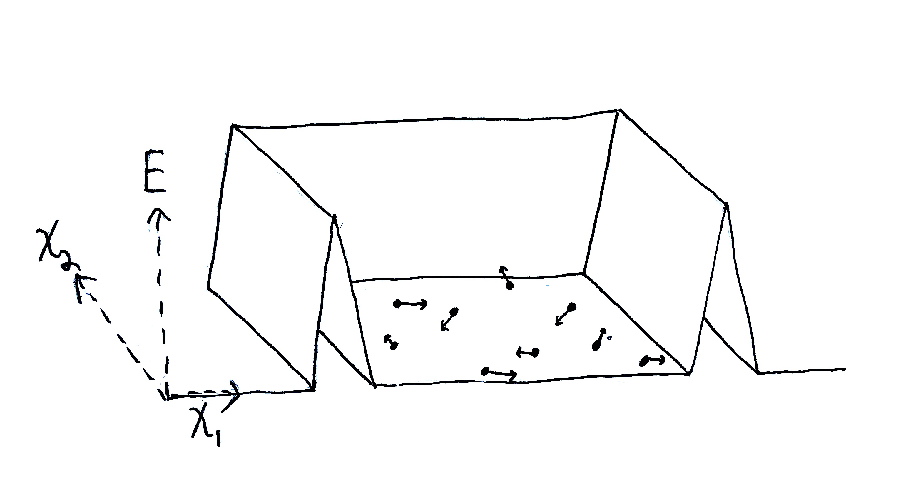
Steep potential hills make up the walls of the box holding a gas.

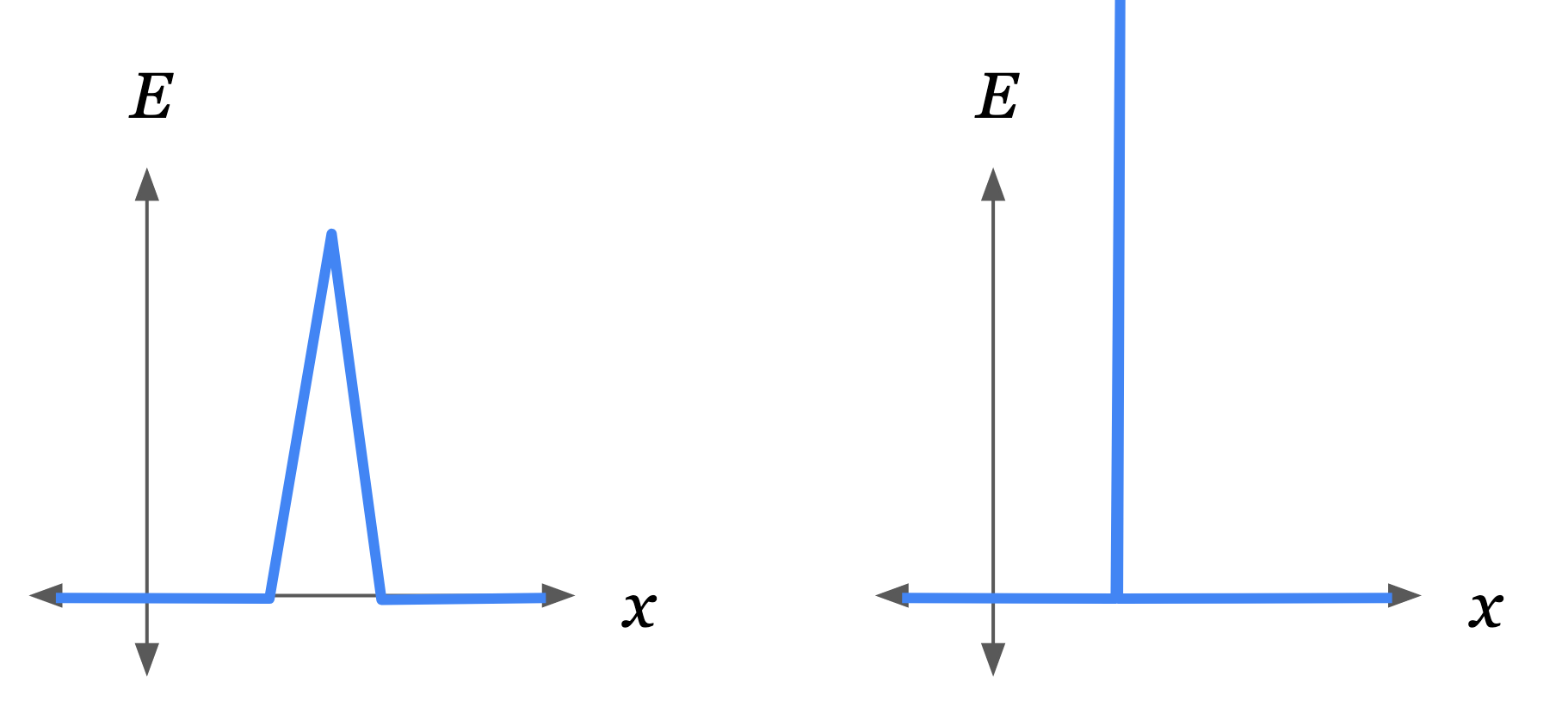
An idealized wall is an infinitely steep and infinitely high potential hill (depicted on the right). This can be constructed by taking the limit of a finite hill (left) as its height goes to infinity and its width goes to zero.

First to describe the forward process on $t=-100$ to $0$, we suppose the container is fixed (external potential $\Ue$ is a constant field) for time $t \in (-\infty,-100)$. At time $t=-100$ the system is in an equilibrium state at temperature $T$ and approximately uniformly filling the container (with some spatial volume $V$). The set of all such states at time $-100$ is the state region $\L\up{1}$. Formally, let $\L\up{1}$ be the set of all positions and momenta of the N particles s.t. the gas is in equilibrium with a constant temperature $T$ and uniformly filling the container. Equilibrium states are those with ergodic trajectories. Specifically, let’s make $\L\up{1}$ the set of all such states which are ergodic over the time interval $(-\infty,-100)$ (i.e. ergodic into the past). Note that specifying that the gas is at temperature $T$ amounts to restricting ourselves to gas states s.t. the average KE is proportional to $T$ (and average KE continues to ergodically bounce around $T$ forever if the container is held fixed).

At time $t=-100$, the container suddenly changes so that its spatial volume increases. This creates a vacuum for the gas to expand into. The gas expands to fill the larger container during the interval $t\in[-100,0]$ (supposing $100$ units of time is enough for the gas to approach close to equilibrium in the larger container). We have that $\Ue$ is also a constant field on the time interval $[-100,0]$. We can determine $\L\up{2}$, the state region at time $t=0$, using a propagator, i.e. $\L\up{2}=\t_{(-100)\to0}(\L\up{1})$.

This forward process is reversible if there exists $\Ue$ defined on the time-interval $(0,\phi]$ s.t. $\t_{0\to\phi}(\L\up{2})=\L\up{1}$. This would be the reverse process.

We know from classical thermodynamics that the forward process from $\L\up{1}$ to $\L\up{2}$ is irreversible. In my naive formulation of the reversibility problem, there is not much we will be able to do with the external potential except to push the particles around. However, pushing particles back to their smaller volume transfers extra KE to them, which means the gas temperature rises (see Szilard Cycle Particle-Piston Interaction Model). One would then have to figure out how to return the extra KE back to the environment.

Example: Isentropic (adiabatic) Expansion

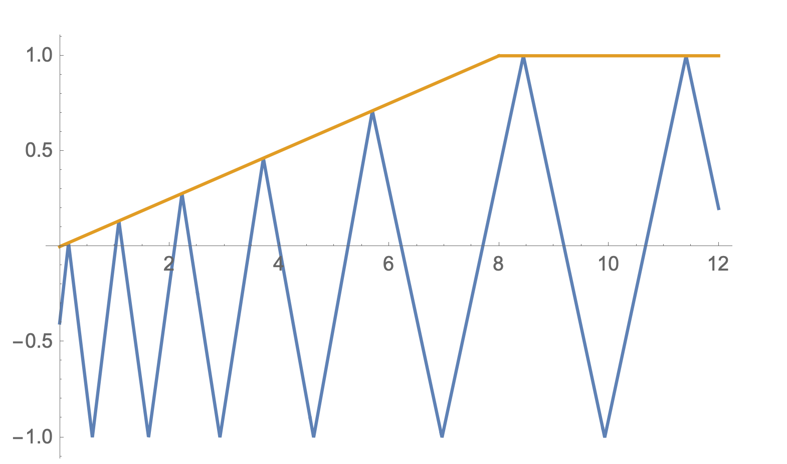
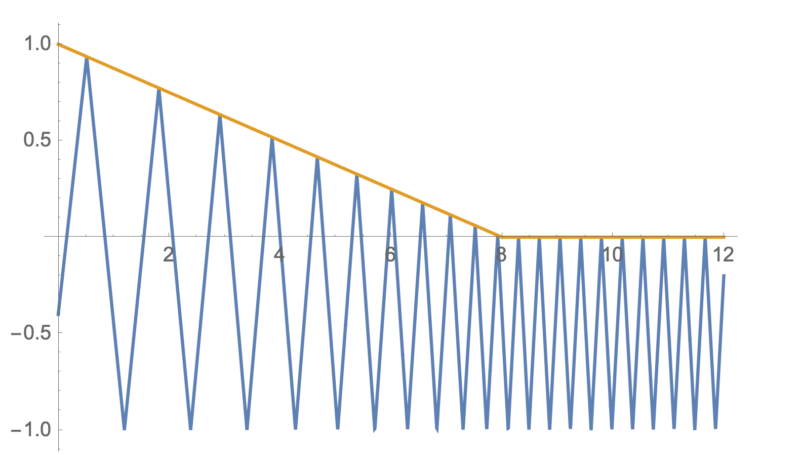
A gas is expanded/compressed by a driven piston. See Szilard Cycle Particle-Piston Interaction Model.

This process trades $q_i$ volume with $p_i$ volume while keeping total state volume fixed. A wall pushing against (compressing) gas particles adds KE to them. A wall pulling away from (expanding) gas particles absorbs KE from them. In classical thermodynamics, this process is reversible.

An example particle trajectory (blue) with a movable wall (orange) moving along a predefined path. Here the wall is moving away from the particle. When the particle collides with the moving wall, the particle loses KE.

An example particle trajectory (blue) with a movable wall (orange) moving along a predefined path. Here the wall is moving towards the particle. When the particle collides with the moving wall, the particle gains KE.

As in the previous example, we let $\L\up{1}$ be the set of states in equilibrium (ergodic infinitely far into the past) at time $t=-100$ with temperature $T$ and spatial volume $V$. $\Ue$ is a fixed field during the time interval $(-\infty,-100)$. On the interval $[-100,0]$, $\Ue$ changes as a function of $t$ s.t. one of the walls of the container pushes or pulls along a fixed trajectory, until reaching its final position at time $t=0$. The resulting potential region is again determined by the propagator $\L\up{2}=\t_{-100\to0}(\L\up{1})$.

Another result from classical thermodynamics is that this process, isentropic expansion/compression, is reversible. One possible reverse process defines $\Ue(\o;\ t)=\Ue(\o;\ -t)$ on the time interval $(0,100]$, so that the wall backtracks its movement from the forward process, returning to its initial position at time $t=-100$.

(Note that an alternative way to model isentropic expansion/compression is to make the moving wall an inertial object with mass, and vary the mass of the wall as a function of its position. See The Carnot Cycle. The wall is now part of the system. By altering the mass function of the wall, the agent drives the process from the outside.)

Issues

I call the above formulation of the reversibility problem naive because,

There are environments and environment interactions which we cannot model.
Energy transfers between different parts of the environment are not accounted for.

Some examples of environments we are not able to model:

Isothermal expansion/compression (requires an infinite heat reservoir).
Environment noise, e.g. thermal noise or shape uncertainty in the container walls of a gas. (see Why Doesn't Uncopying Defeat The 2nd Law?.)
Measurements of system state (the environment gains information about the system’s state). This includes any kind of demon. (see Why Doesn't Uncopying Defeat The 2nd Law? and Why Doesn't Uncopying Defeat The 2nd Law?.)

Heat reservoirs also mess up this formulation of reversibility because irreversible energy transfers between parts of the environment could take place. For instance, in #Example Free Expansion, we could perform isothermal compression to put the gas back into its original container at its original temperature. That means the gas is in thermal contact with a heat reservoir at constant temperature. The energy transferred to the gas as KE during compression is absorbed by the heat reservoir. If the heat reservoir is considered part of the environment, then we are ignoring the conversion of potential energy in the moving wall to heat energy of the reservoir. That distinction is needed for free expansion to be considered irreversible.

Remember, our primary interest is in the reversibility of processes that convert an energy source into useful work. If both the energy source and the thing work is being done to are considered part of the environment, then it wouldn’t make sense to suppose we are indifferent to all the ways energy may be moved around in the environment. It is not enough to suppose that the system is reversed simply if its energy gain/loss is returned to the environment - we care about where in the environment it goes.

Other Formulations

There are two potential avenues towards resolving the above issues with my naive formulation:

Model the environment as part of the system, i.e. model the environment and system together as an isolated parent system.
Model the environment as a conditional potential.

I don’t have an issue-free solution at present. Below I will detail how these two approaches work and their pros and cons.

1. Model environment+system as a joint system

Everything in the outside that has a causal relationship with the system is explicitly modeled in the physics. That is to say, we suppose that the environment has $m$ degrees of freedom, so that the joint state of the system and environment is $\o = (\o_1,\o_2,\dots,\o_{2n+2m}) = (q_1, q_{n+m}, p_1, p_{n+m}) \in \O$. The provided Hamiltonian (and induced propagators) is a function of all the coordinates of both the system and environment.

The Hamiltonian of the joint system must now be time-independent, implying a time-independent external potential term. This allows for some influence from the outside (outside of the environment), but in a limited fashion. The external potential is a sum of fixed (in time) potential fields, so there is no outside to drive the system anymore.

Pros

If we are able to model the physics of the environment, then the definition of reversibility I gave in #Reversibility - Naive Definition works.
We can properly model environment uncertainty (e.g. noise) with a state region on the joint system+environment state space.

Cons

Infinite heat reservoirs require infinite degrees of freedom in the environment, i.e. $m=\infty$. This can easily make the definition of the joint system ill posed (e.g. the Hamiltonian can become infinite).
The system+environment must be otherwise isolated (except for the fixed external potential). That means we cannot model open systems, which is something of particular interest in the thermodynamics of living systems.
The model of the environment needs to be physically accurate. That means no more walls moving along pre-programmed paths (equivalent to inertial walls with infinite mass), like in #Example Isentropic adiabatic Expansion. Also no more discrete degrees of freedom, since all the coordinates must be real-valued and the Hamiltonian must be a smooth function. That means the physical memory bits, like in the Szilard engine (Is The Szilard Cycle Reversible?), must be modeled as some kind of continuous process (e.g. magnets). That can be quite cumbersome.
It is not straightforward to have an outside agent drive the forward and reverse processes, though it is still technically possible. In #Example Isentropic adiabatic Expansion, at the bottom, I briefly mentioned that an agent can drive the interaction between the gas an an inertial wall (movable wall with finite mass whose degree of freedom is included in the Hamiltonian) by modifying the wall’s mass as a function of its position. The generalization of that operation is to modify the Hamiltonian at moments in time, e.g. at time $t$, in a way such that the kinetic energy and potential energy of each $i$-th coordinate is unchanged for states in the state region $\L(t)$ at time $t$. In other words, we are creating a time-dependent Hamiltonian as piecewise (in time) stitching together of time-independent Hamiltonians within various time intervals, so that the boundaries between the piecewise segments have a continuous transition (in this case, all the individual KE and PE for every coordinate is continuously transitioned between Hamiltonians).

2. Model the environment as a conditional potential

A conditional external potential function conditions its own trajectory on the trajectory of the system. There are a few ways to formally define conditional potentials:

$\Ue(\o;\ \s_{(-\infty,t]}, t)$ is a function of the entire history of the system, $\s_{(-\infty,t]} : (-\infty,t]\to\O$, which is a segment of the system’s trajectory defined on the time interval $(-\infty,t]$. Think of this as associating a different trajectory of $\Ue$ to every trajectory of the system. This allows the external potential’s time evolution to condition on what the system is doing, essentially allowing the environment to measure the state of the system. Given an initial state region, the external potential can fork (behave differently for different system trajectories stemming from the state region), resulting in uncertainty on $\Ue$. We could implement environment noise as initial uncertainty on $\Ue$, i.e. we have a set of initial potential functions $\Ue$ as well as an initial state region.

The field-snapshot ${\Ue}\up{t} : \o\mapsto\Ue(\o;\ t)$ is treated as the state of the environment. The propagators time-evolve both system and environment state: $(\o', \Ue') = \t_{t_1\to t_2}(\o, \Ue)$ where $\Ue,\Ue' : \O\to\R$ are time-independent external potentials.
(this is problematic, as entropy may be absorbed into the environment and carried away so that it is no longer reflected in the external potential)

The environment has its own state $\vec{\xi}$.
Let $\vec{q}=(q_1,\dots,q_n)$, $\vec{p}=(p_1,\dots,p_n)$, and $\vec{\xi}$ some state vector for the environment. The environment’s state need not be inertial. $\H(\vec{q},\vec{p};\ \vec{\xi}, t)=T(\vec{p})+\Ui(\vec{q},\vec{p})+\Ue(\vec{q},\vec{p};\ \vec{\xi},t)$, where $\vec{\xi}, t$ are not inertial coordinates involved in Hamilton’s equations (not involved in the physics), but merely specify which external potential to use. ($t$ can be considered part of the environment state, e.g. if someone has a clock.) There is a family of joint propagators of the form $(\vec{q}',\vec{p}', \vec{\xi}') = \t_{t_1\to t_2}(\vec{q},\vec{p}, \vec{\xi})$. We require that the joint propagators be bijections (information preserving). This means than when the environment measures unknown state (conditions on state within the state region), the environment state becomes uncertain. Resetting the system and environment then includes erasing redundant state within the environment. Perhaps something like Landauer’s_principle can be derived from this setup.

Pros

Can get away with modeling less of the environment (only need to model interactions relevant to the system). Don’t care about the state of the universe. Don’t need to reverse literally everything in the universe to reverse the system+environment. E.g. don’t need to reverse things that happened in far away galaxies or wipe the memories of people who know the process occurred.
Can potentially model open environments.

Cons

Reversibility is not longer well defined for open environments because it is not clear what it means for the environment to be reset, i.e. will the environment behave the same every time if its behavior depends on outside state which we are not modeling?
- Boundary between system and environment is not well defined - is a piston part of the system or environment? Anything that cannot be repeated (requires energy that isn’t ambient in the env) is part of the system, like the piston.
Mathematically unwieldy to deal with trajectories of potential fields directly.

What is Entropy?

The use of state regions (subsets of state space) in the formulation of the reversibility problem above looks like Boltzmann’s definition of thermodynamic entropy. Instead of saying “state region”, it is standard to say “macrostate”, which is a set of microstates, i.e. set of fine-grain states, i.e. elements of state space $\O$.

Boltzmann defines the entropy $S$ of a finite macrostate $\L\subseteq\O$ to be

$$
S \propto \log\abs{\L}\,,
$$

i.e. entropy is proportional to the log of the cardinality of $\L$.

For infinite $\L$, we need a measure on $\O$ (in the measure-theoretic sense, not physical measurement) to give us a way to quantify sizes of state regions (**ahem**, macrostates). Let $\mu : \mc{E} \to \R_{\geq0}$ be a measure on $\O$, i.e. $\mu$ is a function from measurable subsets of $\O$ to their respective sizes (not cardinality, but more like length, area or volume for 1D, 2D or 3D regions). Briefly, $\mc{E}$ is a set of measurable subsets of $\O$, and the tuple $(\O,\mc{E},\mu)$ is called a measure space.

Then Boltzmann entropy takes the general form

$$
S \propto \log\mu(\L)\,.
$$

When $\L$ is finite, we can define $\mu$ to be the counting measure (uses set cardinality as set size) to get back Boltzmann’s definition. I hope to show in another post that this definition of entropy of state regions makes sense in the case of gas thermodynamics.

In statistical thermodynamics, there is a common derivation where state space (positions and momenta) of the system (e.g. gas) is discretized into a finite state space. Then the limit of Boltzmann entropy as the discretization size goes to zero gives the entropy of the continuous system. This is equivalent to choosing a uniform measure on state space.

(However, this does not make the choice of measure unique or objective, since what is considered uniform depends on choice of coordinates. E.g. going from cartesian to polar coordinates alters what is considered a uniform measure on the respective coordinate spaces. You could argue that the measure should be uniform on physical space, but then there is no unique uniform measure on canonical coordinates which don’t correspond directly to physical space.)

Before this section, no mention of measures on $\O$ is made. The formulation of the reversibility problem above does not require any quantity like entropy, and does not depend on the choice of measure $\mu$ on $\O$. This allows us to avoid a pesky interpretation problem: what does $\mu$ represent and is there a unique most appropriate choice of $\mu$ for a given system? One could say that side-stepping this issue is necessary for dealing with non-equilibrium (ir)reversibility in general.

The formulation above considers state regions of $\O$ for a single system. In thermodynamics it is often the case that you might consider the separate entropies of multiple different systems (including the environment), and it is common to talk about one system transferring entropy to another. Supposing the state space $\O$ contains multiple systems (each system is described by a subset of coordinate indices) and we have a state region $\L\subseteq\O$ and measure $\mu$ on $\O$, what is the entropy of each system? I propose that the entropy of a system described by coordinates $(\o_i,\dots,\o_j)$ is the log-measure of the projection of $\L$ onto $(\o_i,\dots,\o_j)$, i.e. $S\up{i,\dots,j} \propto \log\mu\Big(\bigcup\set{[\o]_{i,\dots,j}\mid\o\in\L}\Big)$ where $S\up{i,\dots,j}$ is the entropy of the subsystem occupying coordinates $i,\dots,j$, and $[\o]_{i,\dots,j}=\set{\zeta \in \O \mid (\zeta_i,\dots,\zeta_j)=(\o_i,\dots,\o_j)}$ is the set of all states sharing the coordinates $(\o_i,\dots,\o_j)$.

I hope to write more about what justifies this definition of entropy in a future post: .

The Interpretation of State Regions

I briefly mentioned a generalized problem at the bottom of #Reversibility - Naive Definition. To recap, given $\O$, $T$, $\Ui$, $\L_i$ (initial) and $\L_f$ (final), does there exist time interval $\Dt$ and $\Ue$ defined on $[t,t+\Dt]$ s.t. $\L_f=\t_{t\to t+\Dt}(\L_i)$ ?

The chosen state regions are seemingly agent-specific, i.e. are dependent on an agent’s goals. We could characterize them in the following way: $\L_i$ represents what the agent knows, and $\L_f$ represents what the agent wants to have happen in the future.

Given $\L_i$ and $\L_f$, whether there exists a process (specified by $\Ue$) that transforms $\L_i$ to $\L_f$ should be objective, i.e. is a question about physics with a well defined answer. The same is true with the reversibility question: when what is considered successful reversal is defined, the question of whether its achievable has an objective answer.

A further note, the agent’s state of information, $\L_i$, is not subjective or arbitrary. For instance, if the agent posits to know the state of the system to higher resolution then they actually do, the reliable repeatability of the transformation from states in $\L_i$ to states in $\L_f$ will not bear out in practice. Though, the agent could disregard information they have and make $\L_i$ larger than the state region representing what they know, the agent cannot pretend to have more information than they do.

The general problem of reliably transforming $\L_i$ to $\L_f$ is essentially what intelligent systems (agents) try to solve. Agents seek to control their environments. That means causing changes in their environments (i.e. taking actions) so that those environments tend towards desired states. In this way, the generalization of reversibility is controllability. That too would seem to be an objective property of physical systems, once the goal of the agent is defined.

The Reversibility Problem