[This is an article, which is something I’ve optimized for readability and transmission of ideas, opposed to notes that are the seed of an idea and something I’ve written quickly.]

Shannon’s theory of information is usually just called information theory, but is it deserving of that title? Does Shannon’s theory completely capture every possible meaning of the word information? In the grand quests to creating AI and understanding the rules of the universe (i.e. grand unified theory) information may be key. Intelligent agents search for information and manipulate it. Particle interactions in physics may be viewed as information transfer. The physics of information may be key to interpreting quantum mechanics and resolving the measurement problem.

If you endeavor to answer these hard questions, it is prudent to understand existing so-called theories of information so you can evaluate whether they are powerful enough and to take inspiration from them.

Shannon’s information theory is a hard nut to crack. Hopefully this primer gets you far enough along to be able to read a textbook like Elements of Information Theory. At the end I start to explore the question of whether Shannon’s theory is a complete theory of information, and where it might be lacking.

This post is long. That is because Shannon’s information theory is a framework of thought. That framework has a vocabulary which is needed to appreciate the whole. I attempt to gradually build up this vocabulary, stopping along the way to build intuition. With this vocabulary in hand, you will be ready to explore the big questions at the end of this post.

Self-Information

$$
\newcommand{\and}{\wedge}
\newcommand{\or}{\vee}
\newcommand{\E}{\mathbb{E}}
\newcommand{\R}{\mathbb{R}}
\newcommand{\bm}{\boldsymbol}
\newcommand{\rX}{\bm{X}}
\newcommand{\rY}{\bm{Y}}
\newcommand{\rZ}{\bm{Z}}
\newcommand{\rC}{\bm{C}}
\newcommand{\diff}[1]{\mathop{\mathrm{d}#1}}
\newcommand{\kl}[2]{K\left[#1\;\middle\|\;#2\right]}
$$

I’m going to use non-standard notation which I believe avoids some confusion and ambiguities.

Shannon defines information indirectly by defining quantity of information contained in a message/event. This is analogous how physics defines mass and energy in terms of their quantities.

Let’s define $x$ to be any mathematical object from a set of possibilities $X$. We typically call $x$ a message, but it can also be referred to as an outcome, state, or event depending on the context.

Define $h(x)$ ⊕The standard notation is $I(x)$, but this is easy to confuse with mutual information below. to be the self-information of $x$, which is the amount of information gained by receiving ⊕Receiving here can mean, (1) sampling an outcome from a distribution, (2) storing in memory one of its possible states, or (3) viewing with the mind or knowing to be the case one out of the possible cases. $x$. We will see how a natural definition of $h(x)$ arises from combining these two principles:

Quantity of information is a function only of probability of occurrence.
Quantity of information acts like quantity of bits when applied to computer memory.

Principle (1) constrains $h$ to the form $h(x) = f(p_X(x))$, and we do not yet know what $f$ should be.

To see why, let’s unpack (1): it implies that messages/events must always come from a distribution, which is what provides the probabilities. Say you receive a message $x$ sampled from probability distribution (function) $p_X : X \to [0, 1]$ over a discrete ⊕Assume all distributions are discrete until the continuous section. set $X$. Then (1) is saying that $h$ should only look at the probability $p_X(x)$ and not $x$ itself. This is a reasonable requirement, since we want to define information irrespective of the kind of object that $x$ is.

Principle (2) constrains what $f$ should be: $f(p) = -\log_2 p$ ⊕Though we assume a uniform discrete probability distribution to derive this, we will use this definition of $f$ to generalize the same logic to all probability distributions, which is how we arrive at the final definition of $h$., where $p \in [0, 1]$ is a probability value.

To understand (2), consider computer memory. With $N$ bits of memory there are $2^N$ distinguishable states, and only one is the case at one time. Increasing the number of bits exponentially increases the number of counterfactual states ⊕Number of states you could have stored but didn’t.. In memory terms, receiving a “message” of $N$ bits of memory simply means finding out the state those bits are in. Attaching equal weight to each possibility (i.e. memory state) gives us a special case of the probability distribution we used above ⊕To see the equivalence between these two notions of information, i.e. more rare equals more informative vs number of counterfactual states (or memory capacity), it is useful to think of the probability distribution as a weighted possibility space, and of the memory states as possibilities. to define $h$: the uniform distribution, where there are $2^N$ possible states and the weight of single state is $\frac{1}{2^N} = 2^{-N}$.

Composing $f(p) = -\log_2 p$ with $h(x) = f(p_X(x))$ gives us the full definition of self-information:

$$
h(x) = -\log_2 p_X(x)\,.
$$

Regarding notation

From here on, I will use $h(x)$ as a function of message $x$, without specifying the type of $x$. It can be anything: a number, a binary sequence, a string, etc. $f(p)$ is a function of probabilities, rather than messages. So:

$$\begin{align}
& h : X \to \R^+ \text{ maps from messages to information,} \\
\text{and }& f : [0, 1] \to \R^+ \text{ maps from probabilities to information;}
\end{align}$$

and keep in mind that $h(x) = f(p_X(x))$, so $h$ implicitly assumes ⊕I may sometimes write $h_X$ to make explicit the dependency of $h$ on $p_X$. we have a probability distribution over $x$ defined somewhere.

In some places below I’ve written equations in terms of $f$ rather than $h$ ⊕Allow me the slight verbosity now, as you’d probably have had to pore over verbose definitions if I hadn’t. where I felt it would allow you to grasp things just by looking at the shape of the equation.

Bits, not bits

You can get through the above exposition by thinking in terms of computer bits. Now we part ways from the computer bits intuition. Note that this departure occurs when $p_X(x)$ is not a (negative) integer power of two. $h(x)$ will be non-integer, and very likely irrational. What does it mean to have a fraction of a bit? From here on out, it’s better to think of bits as a unit quantifying information, like Joules for energy or kilogram for mass, rather than a count of physical objects ⊕Specifically a physical medium that stores two distinguishable states, usually labeled “0” and “1”.. We will continue to call the unit of $h(x)$ a bit out of convention. Like the kilogram and Joule, this unit can be regarded as undefined in absolute terms, but its usage gives it semantic meaning.

So then how is $h$ to be understood? What is the intuition behind this quantity? In short, Shannon bits are an analytic continuation of computer bits. Just like how the gamma function extends factorial to continuous values, Shannon bits extend the computer bit to non-uniform distributions over a non-power-of-2 number of counterfactuals. Let me explain these two phrases:

non-power-of-2: We have memory that can store one out of $M$ possibilities, where $M \neq 2^N$. For example, I draw a card from a deck of 52. That card holds $-\log_2 \frac{1}{52} = \log_2 52 \approx 5.70044\ldots$ bits of information. A fractional bit can represent a non-power-of-2 possibility space, and quantifies the log-base conversion factor into base $M$. In this case $-log_{52} x = -\frac{\log_2 x}{\log_2 52}$. Note that it is actually common to use units of information other than base-2. For example a nat is log-base-e, a trit is base-3, and dit or ban is base-10.
non-uniform distributions: Using the deck of cards example, let’s say we draw from a sub-deck containing all cards with the hearts suit. We’ve reduced the possibility space to a subset of a super-space, in this case size 13, and have reduced the information contained in a given card, $-\log_2 \frac{1}{13} \approx 3.70044\ldots$ bits. You can think of this as assigning a weight to each card: 0 for cards we exclude, and $\frac{1}{13}$ for cards we include. If we make the non-zero weights non-uniform, we now have an interpretational issue: what is the physical meaning of these weights? Thinking of this weight as a probability of occurrence is one way to recover physical meaning, but this is not a requirement ⊕And probability may not even be an objective property of physical systems in general.. However, I will call these weights probabilities ⊕The reason we wish to hold sum of weights fixed to 1 is so that we can consider the information contained in compound events which are sets of elementary events. In other words, think of the card drawn from the sub-deck of 13 as a card from any suit, i.e. the set of 4 cards with the same number. The card represents an equivalence class over card number., and the weighted-possibility-spaces distributions, as that is the convention. But keep in mind that these weights do not necessarily represent frequencies of occurrence nor uncertainties. The meaning of probability itself is a subject of debate.

The reason we wish to hold sum of weights fixed to 1 is so that we can consider the information contained in compound events which are sets of elementary events. In other words, think of the card drawn from the sub-deck of 13 as a card from any suit, i.e. the set of 4 cards with the same number. The card represents an equivalence class over card number.

Let’s examine some of the properties of $h$ to build further intuition.

First notice that $f(1) = 0$. An event with a probability of 1 contains no information. If $x$ is certain to occur, $x$ is uninformative. Likewise, $f(p) \to \infty$ as $p \to 0$. If $x$ is impossible, it contains infinite information! In general, $h(x)$ goes up as $p_X(x)$ goes down. The less likely an event, the more information it contains. Hopefully this sounds to you like a reasonable property of information.

Next, we can be more specific about how $h$ goes up as $p_X$ goes down. Recall that $f(p) = -\log_2 p$ and $h(x) = f(p_X(x))$, then

$$
f(p/2) = f(p) + 1\,.
$$

If we halve the probability of an event, we add one bit of information to it. That is a nice way to think about our new unit of information. The bit is a halving of probability. Other units can be defined in this way, e.g. the nat is dividing of probability by Euler’s constant e, the trit is a thirding of probability, etc.

Finally, notice that $f(pq) = f(p) + f(q)$. Or to write it another way: $h(x \and y) = h(x) + h(y)$ iff $x$ and $y$ are independent events, because

$$
\begin{align}
h(x \and y) &= -\log_2 p_{X,Y}(x \and y) \\
&= -\log_2 p_X(x)\cdot p_Y(y) \\
&= -\log_2 p_X(x) - \log_2 p_Y(y)\,,
\end{align}
$$

where $x \and y$ indicates the composite event “$x$ and $y$” ⊕We could either think of $x$ and $y$ as composite events themselves from the same distribution, i.e. $x$ and $y$ are sets of elementary events, or as elementary events from two different random variables which have a joint distribution, i.e, $(x, y) \sim (\rX, \rY)$. I will consider the latter case from here on out, because it is conceptually simpler.. Hopefully this is also intuitive. If two events are dependent, i.e. they causally affect each other, it makes sense that they might contain redundant information, meaning that you can predict part of one from the other, and so their combined information is less than the sum of their individual information. You may be surprised to learn that the opposite can also be true. The combined information of two events can be greater than the sum of their individual information! This is called synergy. More on that in the pointwise mutual information section.

In short, we can derive $f(p) = -\log_2 p$ from (1) additivity of information, $f(pq) = f(p) + f(q)$, and (2) a choice of unit, $f(½) = 1$. Proof.

Recap

To make the full analogy: a weighting over possibilities is like a continuous relaxation of a set. An element is or is not in a set, while adding weights to elements (in a larger set) allows their member ship to have degrees, i.e. the “is element” relation becomes a fuzzy value between 0 and 1 ⊕We recover regular sets by setting all weights to either 0 or uniform non-zero weights.. With a weighted possibility space we have a lot more freedom to work with extra information beyond just merely which possibilities are in the set. Probability distributions are more expressive than mere sets.

Stepping back

The unit bit that we’ve defined is connected to computer bits only because they both convert multiplication to addition.

Computer bits: $(2^N\cdot2^M)$ states $\Longrightarrow$ $(N+M)$ bits.
Shannon bits: $(p\cdot q)$ probability $\Longrightarrow$ $(-\log_2 p - \log_2 q)$ bits.

The way I’ve motivated $h$ is a departure from Shannon’s original motivation for defining self-information, which was to describe the theoretically optimal lossless compression for messages being sent over a communication channel. Under this viewpoint, $h(x)$ quantifies the theoretically minimum possible length (in physical bits) to encode message $x$ in computer memory without loss of information. Under this view, $h(x)$ should be thought of as the asymptotic average bit-length for the optimal encoding of $x$ in an infinite sequence of messages drawn from $p_X$. Hence why it makes sense for $h(x)$ to be a continuous value. For more details, see arithmetic coding.

We are now flipping Shannon’s original motivation on its head, and using the theoretically optimal encoding length in bits as the definition of information content. In the following discussion, we don’t care how messages/events are actually represented physically. Our definition of information only cares about probability of occurrence, and is in fact blind to the contents of messages ⊕Something that could be seen as either a flaw or a virtue, which I discuss below.. The connection of probability to optimal physical encoding is one of the beautiful results that propelled Shannon’s framework into its lofty position as information theory. However, for our purposes, we simply care about defining quantity of information, and do not care at all about how best to compress or store data for practical purposes.

To be clear, when I talk about the self-information of a message, I am not saying anything about how the message is physically encoded or transmitted, and indeed it need not be encoded with an optimal number of computer bits. I am merely referring to a quantified ⊕Hopefully this quantity is objective and measurable in principle - something I discuss below property of the message, i.e. it’s information content. The number of computer bits a message is encoded with need not equal the number of Shannon bits it contains! ⊕In short, physical encoding length and probability of occurrence need not be linked.

Entropy

In the last section I said that under the view of optimal lossless compression, $h(x)$ is the bit length of the optimal encoding for $x$ averaged over an infinite sample from random variable $\rX$, and arithmetic coding can approach this limit. We could also consider the average bit length per message from $\rX$ (averaged across all messages). That is the entropy of random variable $\rX$, which is the expected self-information,

$$
\begin{align}
H[\rX] &= \E_{x\sim \rX}[h(x)] \\
&= \E_{x\sim \rX}[-\log_2\,p_X(x)]\,.
\end{align}
$$

In the quantifying information view, think of entropy $H[\rX]$ as the number of bits you expect to gain by observing an event sampled from $p_X(x)$. In that sense it is a measure of uncertainty, i.e. how much information I do not have, i.e. quantifying what is unknown.

Let’s build our intuition of entropy. A good way to view entropy is as a measure of how spread out a distribution is. Entropy is actually a type of statistical dispersion of $p_X$, meaning you could use it as an alternative to statistical variance.

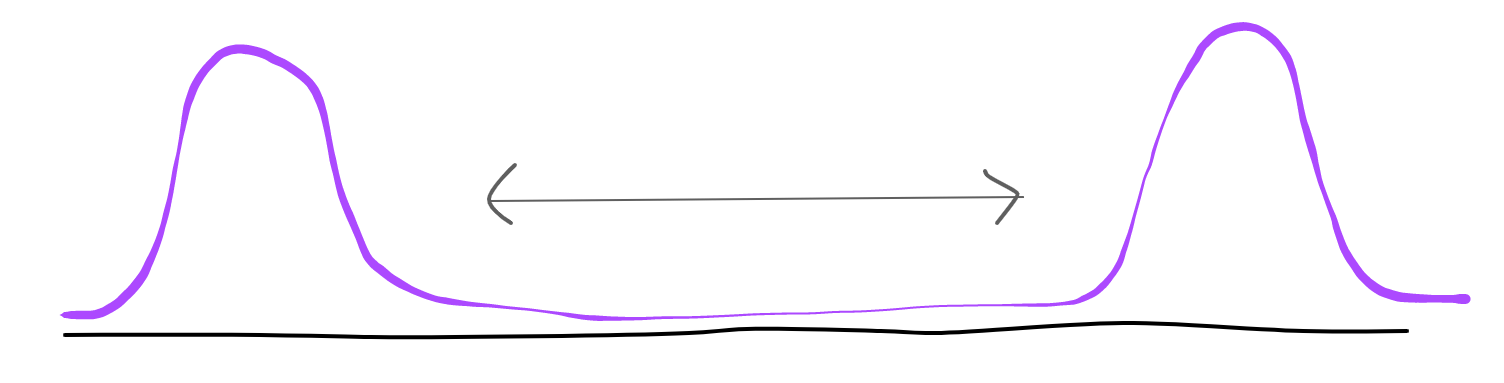For example, a bi-modal distribution can have arbitrarily high variance by moving the modes far apart, but the overall spread-out-ness (entropy) will not necessarily change.

The more spread out a distribution is, the higher its entropy. For bounded support, the uniform distribution has highest entropy (other max-entropy distributions). The minimum possible entropy is 0 ⊕Note that in the expectation, 0-probability outcomes have infinite self-information, so we have to use the convention that $p_X(x)\cdot h(x) = 0\cdot\infty = 0$., which indicates a deterministic distribution, i.e. $p_X(x) \in \\{0, 1\\}$ for all $x \in X$.

Credit: https://en.wikipedia.org/wiki/Binary_entropy_function

Though Shannon calls his new idea entropy, the connection to physical entropy is nontrivial. If there is a connection, that is more of a coincidence. Apparently Shannon’s decision to call it entropy was made by a suggestion by von Neumann at a party: http://www.eoht.info/page/Neumann-Shannon+anecdote
[credit: Mark Moon]

There are connections between information entropy and thermodynamics entropy (see https://plato.stanford.edu/entries/information-entropy/), but I do not yet understand them well enough to give an overview here - perhaps in a future post. Some physicists consider information to have a physical nature, and even a conservation law ⊕In the sense that requiring physics be time-symmetric is equivalent to requiring information to be conserved.! Further reading: The Theoretical Minimum - Entropy and conservation of information, no-hiding theorem.

Question: Why expected self-information?
We could have used median or something else. Expectation is a default go-to operation over distributions ⊕See my previous post: http://zhat.io/articles/bias-variance#bias-variance-decomposition-for-any-loss because of its nice properties, but ultimately it is an arbitrary choice. However, as we will see, one huge benefit in our case is that expectation is linear.

Regarding notation

From here on out, I will drop the subscript $X$ from $p_X(x)$ when $p(x)$ unambiguously refers to the probability of $x$. This is a common thing to do, but it can also lead to ambiguity if I want to write $p(0)$, the probability that $x$ is 0. A possible resolution is to use random variable notation, $p(\rX = 0)$, which I use in some places. However, there is the same issue for self-information. For example, quantities $h(x), h(y), h(x\and y), h(y \mid x)$. I will add subscripts to $h$ when it would be ambiguous otherwise, for example $h_X(0), h_Y(0), h_{X,Y}(x\and y), h_{Y\mid X}(0 \mid 0)$ .

Conditional Entropy

Conditional self-information, defined as

$$
\begin{align}
h(y \mid x) &= -\log_2\,p(y \mid x)\\
&= -\log_2(p(y \and x) / p(x)) \\
&= h(x \and y) - h(x)\,,
\end{align}
$$

is the information you stand to gain by observing $y$ given that you already observed $x$. I let $x \and y$ denote the observation of $x$ and $y$ together (I could write $(x, y)$, but then $p((y, x))$ would look awkward).

If $x$ and $y$ are independent events, $h(y \mid x) = h(y)$. Otherwise, $h(y \mid x)$ can be greater or less than $h(y)$. It may seem counterintuitive that $h(y \mid x) > h(y)$ can happen, because this implies you gain more from $y$ by just simply knowing something else, $x$. However, this reflects the fact that you are unlikely to see $x, y$ together. Likewise, if $h(y \mid x) < h(y)$ you are likely to see $x, y$ together. More on this in the next section.

Confusingly, conditional entropy can refer to two different things.

First is expected conditional self-information,

$$
\begin{align}
H[\rY \mid \rX = x] &= \E_{y\sim \rY \mid \rX=x}[h(y \mid x)] \\
&= \E_{y\sim \rY \mid \rX=x}[\log_2\left(\frac{p(x)}{p(x, y)}\right)] \\
&= \sum\limits_{y \in Y} p(y \mid x) \log_2\left(\frac{p(x)}{p(x, y)}\right)\,.
\end{align}
$$

The other is what is most often referred to as conditional entropy,

$$
\begin{align}
H[\rY \mid \rX] &= \E_{x,y \sim \rX,\rY}[h(y \mid x)] \\
&= \E_{x,y \sim \rX,\rY}[\log_2\left(\frac{p(x)}{p(x, y)}\right)] \\
&= \E_{x\sim \rX} H[\rY \mid \rX = x]\,.
\end{align}
$$

The intuition behind $H[\rY \mid \rX = x]$ will be the same as of entropy, $H[\rY]$, which we covered in the last section. Let’s gain some intuition for $H[\rY \mid \rX]$. If $H[\rY]$ measures uncertainty of $\rY$, then $H[\rY \mid \rX = x]$ measures conditional uncertainty given $x$, and $H[\rY \mid \rX]$ measures average conditional uncertainty w.r.t. $\rX$.

The maximum value of $H[\rY \mid \rX]$ is $H[\rY]$, which is achieved when $\rX$ and $\rY$ are independent random variables. This should make sense, as recieving a message from $\rX$ does not tell you anything about $\rY$, so your state of uncertainty does not decrease.

The minimum value of $H[\rY \mid \rX]$ is 0, which is achieved when $p_{\rY \mid \rX}(\rY \mid \rX = x)$ is deterministic for all $x$. In other words, you can define a function $g : X \rightarrow Y$ to map from $X$ to $Y$. This wouldn’t otherwise be the case when $\rY \mid \rX$ is stochastic.

$H[\rY \mid \rX]$ is useful because it takes all $x \in X$ into consideration. You might have, for example, $H[\rY \mid \rX = x_1] = 0$ for $x_1$, but $H[\rY \mid \rX] > 0$, which means $y$ cannot always be deterministically decided from $x$. In the section on mutual information we will see how to think of $H[\rY \mid \rX]$ as a property of a stochastic function from $X$ to $Y$.

Because of linearity of expectation, all identities that hold for self-information hold for their entropy counterparts. For example,

$$
\begin{align}
h(y \mid x) &= h(x \and y) - h(x) \\
\Longrightarrow H[\rY \mid \rX] &= H[(\rX, \rY)] - H[\rX]\,.
\end{align}
$$

This is a nice result. This equation says that the average uncertainty about $\rY$ given $\rX$ ⊕Amount of information left to observe in $\rY$ on average. equals the total expected information in their joint distribution, $(\rX, \rY)$, minus the average information in $\rX$. In other words, conditional entropy is the total information in $x \and y$ minus information in what you have, $x$, all averaged over all the possible $(x, y)$ you can have.

Mutual Information

In my view, mutual information is what holds promise as a definition of information. This it the most important topic to understand for tackling the problems with Shannon information section below.

Pointwise Mutual Information

When two events $x$ and $y$ are dependent, how do we compute their total information? Previously we said that $h(x \and y) = h(x) + h(y)$ iff $p_X(x \and y) = p_X(x)p_X(y)$. However, the general case is,

$$
h(x \and y) = h(x) + h(y) - i(x, y)\,,
$$

where I am defining $i(x, y)$ such that this equation holds. Rearranging we get

$$
\begin{align}
i(x, y) &= h(x) + h(y) - h(x \and y) \\
&= -\log_2(p_X(x)) - \log_2(p_X(y)) + \log_2(p_X(x \and y)) \\
&= \log_2\left(\frac{p_X(x, y)}{p_X(x)p_X(y)}\right)\,.
\end{align}
$$

$i(x, y)$ is called pointwise mutual information (PMI). Informally, PMI measures the amount of bits shared by two events. To say that another way, it measures how much information I have about one event given I only observe the other. Notice that PMI is symmetric, $i(x, y) = i(y, x)$, so any two events contain the same information about each other.

$i(x, y)$ is a difference in information. Positive $i(x, y)$ indicates redundancy, i.e. total information is less than the sum of the parts ⊕If you object that it doesn’t make sense to lose information by observing $x$ and $y$ together over observing them separately, it is important to note that $h(x) + h(y)$ is not a physically meaningful quantity, unless they are independent. Technically, you would have $h(x) + h(y \mid x)$ in total. $h(x)$ and $h(y)$ are both the amounts of information to gain by observing either $x$ or $y$ first.: $h(x, y) < h(x) + h(y)$. However, it may also be the case that $i(x, y)$ is negative so that $h(x, y) > h(x) + h(y)$. This is called synergy. ⊕The word synergy is conventionally used in the context of expected mutual information, and I am running the risk of conflating two distinct phenomenon under the same word. There is no synergy among two random variables under expected mutual information, and this type of synergy only appears among 3 or more random variables. See https://en.wikipedia.org/wiki/Multivariate_mutual_information#Synergy_and_redundancy.

This is highly speculative, but synergy (either the pointwise-MI or expected-MI kind) may be a fundamental insight that could explain emergence ⊕Emergence is a concept in philosophy. See https://en.wikipedia.org/wiki/Emergence and https://plato.stanford.edu/entries/properties-emergent/ and possible limitations of reductionism in illuminating reality. See Higher-level causation exists (but I wish it didn’t).

Example:
Let $X = \\{0, 1\\}$ and $Y = \\{0, 1\\}$, then the joint sample space is the cartesian product $X \times Y$. $p_X(x), p_Y(y)$ denote marginal probabilities, and $p_{X,Y}(x, y)$ is their joint probability. The joint probability table:

$x$	$y$	$p_{X,Y}(x, y)$
0	0	1/16
0	1	7/16
1	0	7/16
1	1	1/16

We have

$h_X(0) = -\log_2 p_X(0) = -\log_2 1/2 = 1$
$h_Y(0) = -\log_2 p_Y(0) = -\log_2 1/2 = 1$
$h_{X,Y}(0 \and 0) = -\log_2 p_{X,Y}(0, 0) = -\log_2 1/16 = 4$

$i(0,0) = h_X(0) + h_Y(0) - h_{X,Y}(0 \and 0) = -2$, and so $(0,0)$ is synergistic. On the other hand, $i(0,1) \approx 0.80735$, indicating $(0,1)$ is redundant.

Properties of PMI

Let’s explore some of the properties of PMI. From here on out, I will consider sampling elementary events from a joint distribution, $(x, y) \sim (\rX, \rY)$, where $\rX, \rY$ are unspecified discrete (possibly infinite) random variables. For notational simplicity I’ll drop the subscripts from distributions, so $p(x), p(y)$ denote the marginals, $\rX$ and $\rY$ respectively, and $p(x, y)$ denotes the joint $(\rX,\rY)$.

To recap, PMI measures the difference in bits between the product of marginals $p(x)p(y)$ and the joint $p(x, y)$, as evidenced by

$$
\begin{align}
i(x, y) &= \log_2\left(\frac{p(x, y)}{p(x)p(y)}\right) \\
&= h(x) + h(y) - h(x \and y)\,.
\end{align}
$$

Negative PMI implies synergy, while positive PMI implies redundancy.

Another way to think about PMI is as a measure of how much $p(y \mid x)$ differs from $p(y)$ (and vice versa). Suppose an oracle sampled $(x, y) \sim (\rX,\rY)$, but the outcome $(x, y)$ remains hidden from you. $p(y)$ is the information you stand to gain by having $y$ revealed to you. However, $p(y \mid x)$ is what you stand to gain from seeing $y$ if $x$ is already revealed. You do not know how much information $x$ contains about $y$ without seeing $y$. Only the oracle knows this. However, if you know $p(y \mid x)$, then you can compute your expected information gain (conditional uncertainty), $H[\rY \mid \rX=x]$.

PMI measures the change in information you will gain about $y$ (from the oracle’s perspective) before and after $x$ is revealed (and vice versa). In this view, it makes sense to rewrite PMI as

$$
\begin{align}
i(x, y) &= \log_2\left(\frac{p(y \mid x)}{p(y)}\right) \\
&= -\log_2\,p(y) + \log_2\,p(y \mid x) \\
&= h(y) - h(y \mid x)\,.
\end{align}
$$

Special Values

By definition, $i(x, y) = 0$ iff $\rX, \rY$ are independent. Verifying, we see that,

$$
\begin{align}
i(x, y) &= \log_2\left(\frac{p(x)p(y)}{p(x)p(y)}\right) \\
&= 0\,.
\end{align}
$$

The maximum possible PMI happens when $x$ and $y$ are perfectly associated, i,e. $p(y \mid x) = 1$ or $p(x \mid y) = 1$. So $h(y \mid x) = 0$ or vice versa, meaning you know everything about $y$ if you have $x$. Then $i(x, y) = h(y) - h(y \mid x) = h(y)$. In general, the maximum possible PMI is $\min\\{h(x), h(y)\\}$.

PMI has no minimum, and goes to $-\infty$ if $x$ and $y$ can never occur together but can occur separately, i.e. $p(x, y) = 0$ while $p(x), p(y) > 0$. We can see that $p(y \mid x) = p(x, y)/p(x) = 0$ so long as $p(x) > 0$. So $h(y \mid x) \to \infty$, and we have $i(x, y) = h(y) - h(y \mid x) \to -\infty$ if $h(y) > 0$.

While redundancy is bounded, synergy is infinite. This should make sense, as $h(x), h(y)$ are bounded so there is a maximum amount of information to redundantly share. On the other hand, synergy measures how rare the co-occurrence of $(x,y)$ together are, relative to their marginal probabilities, where lower $p(x, y)$ means their co-occurrence is more special. So if $(x,y)$ can never occur, then their co-occurrence is infinitely special.

Expected Mutual Information

Expected mutual information, also just called mutual information (MI), is given as

$$
\begin{align}
I[\rX, \rY] &= \E_{x\sim X, y\sim Y}[i(x, y)] \\
&= \E_{x\sim X, y\sim Y}\left[\log_2\left(\frac{p(x, y)}{p(x)p(y)}\right)\right]\,.
\end{align}
$$

$I$ is to correlation as $H$ is to variance. While correlation measures to what extent $\rX$ and $\rY$ have a linear relationship, $I$ measures the strength of their statistical dependency. While variance measures average distance from some critical point, $H$ is distance agnostic, i.e. it measures unordered dispersion. Similarly, while statistical correlation measures deviation of the mapping between $\rX$ and $\rY$ from perfectly linear, $I$ is shape agnostic, i.e. it measures unordered causal dependence.

First off, it is important to point out that $I$ is always non-negative, unlike its pointwise counterpart (proof here). You can see this intuitively by trying to construct an anti-dependent relationship between $\rX$ and $\rY$. On average, $p(x, y)$ would have to be less than the product of their marginals. You can construct individual cases where this is true for a particular $(x, y)$, but to do that, you will have to fill most of the probability table (for 2D joint) with p-mass to compensate. This is reflected in Jensen’s inequality. A direct consequence is $H[\rY] \geq H[\rY \mid \rX]$.

$I$ being non-negative means you can safely think about it as a measure of information content. In this sense, information is stored in the relationship between $\rX$ and $\rY$.

Note that by remembering that expectation is linear, some useful identities pop out of the definition above,

$$
\begin{align}
I[\rX, \rY] &= H[\rX] + H[\rY] - H[(\rX,\rY)] \\
&= H[\rX] - H[\rX \mid \rY] \\
&= H[\rY] - H[\rY \mid \rX]\,.
\end{align}
$$

An intuitive way to think about $I$ is as a continuous measure of bijectivity of the stochastic function, $g(x) \sim p(\rY \mid \rX = x)$, where $g : X \rightarrow Y$. This is easier to see if we write

$$
I[\rX, \rY] = H[\rY] - H[\rY \mid \rX]\,.
$$

$H[\rY]$ measures surjectivity, i.e. how much $g$ spreads out over $Y$ (marginalized over $\rX$). surjective (a.k.a. onto) in the set-theory sense means that $g$ maps to every element in $Y$. In the statistical sense, $g$ may map to every element in $Y$ with some probability, but to some elements much more frequently than others. We would say $p(y)$ is peaky, the opposite of spread out. Recall that $H$ measures statistical dispersion. Larger $H[\rY]$ means more even spread of probability mass across all the elements in $Y$. In that sense, it measures how surjective $g$ is.

$H[\rY \mid \rX]$ measures anti-injectivity. injective (a.k.a. one-to-one) in the set-theory sense means that $g$ maps every element in $X$ to a unique element in $Y$. There is no sharing, and you know which $x \in X$ was the input for any $y \in Y$ in the image of $g(X)$. In the statistical sense, $g$ may map a given $x$ to many elements in $Y$, each with some probability, i.e. fan-out. Anti-injective is like a reversal of injective, which is about fan-in. The more $g$ fans-out, the more anti-injective it is. Recall that $H[\rY \mid \rX]$ measures averge uncertainty about $\rY$ given an observation from $\rX$. This is, in a sense, the average statistical fan-out of $g$. Lower $H[\rY \mid \rX]$ means $g$’s output is more concentrated (peaky) on average for a given $x$, and higher means its output is more uniformly spread on average.

For a function to be a bijection, is needs to be both injective and surjective. $H[\rY]$ may seem like a good continuous proxy for surjectivity, but $H[\rY \mid \rX]$ seems to measure something different from injectivity. Notice that $H[\rY \mid \rX]$ is affected by the injectivity of $g^{-1}$. If $g^{-1}$ maps many $y$s to the same $x$, then we are uncertain about what $g(x)$ should be.

In general, I claim that $I[\rX, \rY]$ measures how bijective $g$ is. $I[\rX, \rY]$ is maximized when $H[\rY]$ is maximized and $H[\rY \mid \rX]$ is minimized (i.e. 0). That is, when $g$ is maximally surjective and minimally anti-injective, implying it is maximally injective. Higher $I[\rX, \rY]$ actually does indicate that $g$ is more invertible because $I$ is symmetric. It measures how much information can flow through $g$ in either direction.

Useful diagram for keeping track of the relationships between these concepts.
Credit: https://en.wikipedia.org/wiki/Mutual_information

Channel capacity

$I$ is determined by $p(x)$ just as much as $p(y \mid x)$, but $g$ has ostensibly nothing to do with $p(x)$. If we want $I$ to measure properties of $g$ in isolation, it should not care about the distribution over its inputs. One solution to this issue is to use the capacity of $g$, defined as

$$
\begin{align}
C[g] &= \sup_{p_X(x)} I[\rX, \rY] \\
&= \sup_{p_X(x)} \E_{y\sim p_{g(x)}, x \sim p_X}[i(x, y)] \\
&= \sup_{p_X(x)} \E_{y\sim p_{Y \mid X=x}, x \sim p_X}[-h(y \mid x) + h(x)]\,.
\end{align}
$$

In other words, if you don’t have a preference for $p(x)$, choose $p(x)$ which maximizes $I[\rX, \rY]$.

Shannon Information For Continuous Distributions

Up to now we’ve only considered discrete distributions. Describing the information content in continuous distributions and their events is tricky business, and a bit more nuanced than usually portrayed. Let’s explore this.

For this discussion, let’s consider a random variable $\rX$ with support over $\R$. Let $f(x)$ be the probability density function (pdf) of $\rX$.

Elementary events $x \in \R$ do not have probabilities perse ⊕you could say their probability mass is 0 in the limit. Self-information is a function of probability mass, so we should instead compute self-info of events that are intervals (or measurable sets) over $\R$. For example,

$$
\begin{align}
h(a < x < b) &= -\log_2\,p(a < \rX < b)\\
&= -\log_2\left(\int_a^b f(x) \diff x\right)
\end{align}
$$

Conjecture: The entropy of any distribution with uncountable support is infinite. This should make sense, as we now have uncountably many possible outcomes. One observation rules out infinitely many alternatives, so it should contain infinite information. We can see this clearly because the entropy of a uniform distribution over $N$ possibilities is $\log_2 N$ which grows to infinity as $N$ does. On the other hand, a one-hot distribution over $N$ possibilities has 0 entropy, because you will always observe ⊕Unless you observe an impossible outcome, in which case you gain infinite information! the probability-1 outcome and gain 0 information. So we expect the Dirac-delta distribution to have 0 entropy.

But wait, the Gaussian distribution is a maximum-entropy distribution. That people can say “a continuous distribution has maximum entropy” implies their entropies can be numerically compared! And frankly, people talk about entropy of continuous distributions all the time, and they are very much finite! It turns out, what people normally call entropy for continuous distributions is actually differential entropy, which is not the same thing as the $H$ we’ve been working with.

I’ll show that $H[\rX]$ is infinite when the distribution has continuous support, following a similar proof in Introduction to Continuous Entropy ⊕And also in Elements of Information Theory section 8.3.. To do that, let’s take a Riemann sum of $f(x)$. Let $\\{x_i\\}_{i=-\infty}^\infty$ be a set of points equally spaced by intervals of $\Delta$.

$$
% \def\u{\Delta x}
\def\u{\Delta}
\begin{align}
H[\rX] &= -\lim\limits_{\u \to 0} \sum\limits_{i=-\infty}^\infty f(x_i) \u \log_2\left(f(x_i) \u\right) \\
&= -\lim\limits_{\u \to 0} \sum\limits_{i=-\infty}^\infty f(x_i) \u \log_2\left(f(x_i)\right) - \lim\limits_{\u \to 0} \sum\limits_{i=-\infty}^\infty f(x_i) \u \log_2\left(\u\right)\,.
\end{align}
$$

The left term is just the Riemann integral of $f(x)\log_2(f(x))$, which I will define as differential entropy ⊕Typically $h$ is used to denote differential entropy, but I’ve already used it for self-information, so I’m using $\eta$ instead.:

$$
\eta[f] := -\lim\limits_{\u \to 0} \sum\limits_{i=-\infty}^\infty f(x_i) \u \log_2\left(f(x_i)\right) = -\int_{-\infty}^\infty f(x) \log_2\left(f(x)\right) \diff{x}\,.
$$

The right term can be simplified using the limit product rule:

$$
-\lim\limits_{\u \to 0} \sum\limits_{i=-\infty}^\infty f(x_i) \u \log_2\left(\u\right) = -\left(\lim\limits_{\u \to 0} \sum\limits_{i=-\infty}^\infty f(x_i) \u\right)\cdot\left(\lim\limits_{\u \to 0}\log_2\left(\u\right)\right)\,.
$$

Note that

$$
\lim\limits_{\u \to 0} \sum\limits_{i=-\infty}^\infty f(x_i) \u = \int_{-\infty}^\infty f(x) \diff{x} = 1\,,
$$
because $f(x)$ is a p.d.f.

Putting it all together we have

$$
H[\rX] = \eta[f] - \lim\limits_{\u \to 0}\log_2\left(\u\right)\,.
$$

$\log_2(\u) \to -\infty$ as $\u \to 0$, so $H[\rX]$ explodes to infinity when $\eta[f]$ is finite, which it is for most well-behaved functions.

A simple proof that $H$ is finite for continuous distributions with support over an finite set: the Riemann sum above will only have at most finitely many non-zero terms as $\Delta \to \infty$.

Differential entropy is very different from entropy. It can be unboundedly negative. For example, the differential entropy of a Gaussian distribution with variance $\sigma^2$ is $\frac{1}{2}\ln(2\pi e \sigma^2)$. Taking the limit as $\sigma \to 0$, we see the differential entropy of the Dirac-delta distribution is $-\infty$ ⊕Plugging $\eta[f] = -\infty$ into our relation $H[\rX] = \eta[f] - \lim\limits_{\u \to 0}\log_2\left(\u\right)$, we see why entropy of $\delta(x)$ would be 0.. A notable problem with differential entropy is that its not invariant to change of coordinates, and there is a proposed fix for that: https://en.wikipedia.org/wiki/Limiting_density_of_discrete_points.

Proof that MI is fininte for continuous distributions

A very nice result is that expected mutual information is finite where entropy would be infinite, so long as there is some amount of noise between the two random variables. This implies that even if physical processes are continuous and contain infinite information, we can only get finite information out of them, because measurement requires establishing a statistical relation between the measurement device and that system which is always noisy in reality. MI is agnostic to discrete or continuous universes! As long as there is some amount of noise in between a system and your measurement, your measurement will contain finite information about the system.

The proof follows the same Riemann sum approach from the previous section. I will show that mutual information and differential mutual information are equivalent. Since differential mutual information finite for well behaved functions, so is mutual information!

$$
\begin{align}
I[\rX, \rY] &= -\lim\limits_{\u \to 0} \sum\limits_{i=-\infty}^\infty \sum\limits_{j=-\infty}^\infty f_{XY}(x_i, y_j) \u^2 \log_2\left(\frac{f_{XY}(x_i, y_j)\u^2}{f_X(x_i)\u f_Y(y_i)\u} \right) \\
&= -\lim\limits_{\u \to 0} \sum\limits_{i=-\infty}^\infty \sum\limits_{j=-\infty}^\infty f_{XY}(x_i, y_j) \u^2 \log_2\left(\frac{f_{XY}(x_i, y_j)}{f_X(x_i)f_Y(y_i)} \right) \\
&= \int_{-\infty}^\infty \int_{-\infty}^\infty f_{XY}(x_i, y_j) \log_2\left(\frac{f_{XY}(x_i, y_j)}{f_X(x_i)f_Y(y_i)} \right) \diff{y}\diff{x}\,
\end{align}
$$

because the $\Delta$s cancel inside the log.

If $p(\rY \mid \rX = x)$ is a Dirac-delta for all $x$, and $p(\rY)$ has continuous support, then $I[\rX, \rY]= H[\rY] - H[\rY \mid \rX] = \infty$ because $H[\rY]=\infty$ and $H[\rY \mid \rX]=0$. Thus some noise between $\rX$ and $\rY$ is required to make the MI finite. It follows that $I[\rX, \rX] = H[\rX] = \infty$ when $\rX$ has continuous support.

Problems With Shannon Information

Question: Do the concepts just outlined capture our colloquial understanding of information? Are there situations where they behave differently from how we expect information to behave? I’ll go through some fairly immediate objections to this Shannon’s definition of information, and some remedies.

1. TV Static Problem

Imagine a TV displaying static noise. If we assume a fairly uniform distribution over all “static noise” images, we know that the entropy of the TV visuals will be high, because probability mass is spread fairly evenly across all possible images. Each image on average has a very low probability of occurring. According to Shannon, each image then contains a large amount of information.

That may sound absurd. Noise, by some definitions, carries no useful information. Noise is uninformative. To a human looking at TV static, the information gained is that the TV is not displaying anything. This is a very high level piece of information, but much less than the supposedly high information content of the static itself.

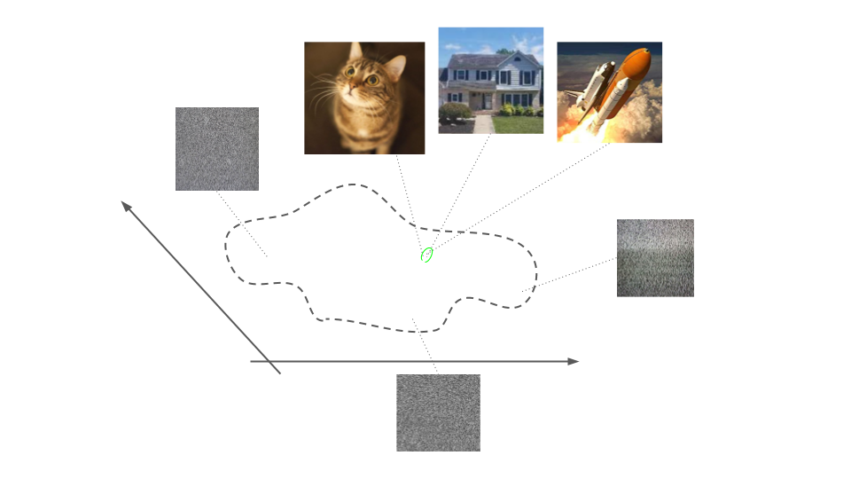
The resolution here is to define what it means for a human to obtain information. I propose looking at the mutual information between the TV and the viewer’s brain. Let $\rX$ be a random variable over TV images, and $\rZ$ be a random variable over the viewer’s brain states. The support of $\rX$ is the space of all possible TV screens, so static and SpongeBob are just different distributions over the same space. Now, the state of the viewer’s brain is causally connected to what is on the TV screen, but the nature of their visual encoder (visual cortex) determines $p(\rZ \mid \rX)$, and thus $p(\rZ, \rX)$. I would guess that any person who says TV static is uninformative does not retain much detail about the patterns in the static. Basically, that person would just remember that they saw static. What we have here is a region of large fan-in. Many static images are collapsed to a single output for their visual encoder, namely the label “TV noise”. So the information contained in TV static is low to a human, because $I[\rX, \rZ]$ is low when $\rX$ is the distribution of TV static.

Note that the signal, “TV noise”, is still rather informative, if you consider the space of all possible labels you could assign to the TV screen, e.g. “SpongeBob” or “sitcom”. Further, that you are looking at a TV and not anything else is information.

Encryption scrambles information to make it inaccessible to prying eyes. Encryption is usually lossless, meaning the original message is fully recoverable. If $\rX$ is a distribution over messages, then the encryption function Enc should preserve that distribution. To Shannon information, $\rX$ and $\text{Enc}(\rX)$ contain the same information. Shannon information is therefore blind to operations like scrambling which do something interesting to the information present, i.e. like making it accessible or inaccessible.

The resolution is again mutual information. While permuting message space (or any bijective transformation) does not change information content under Shannon, it changes the useful information content. A human looking at (or otherwise perceiving) a message is creating a casual link between the message and a representation in the brain. This link has mutual information. Likewise, any measurement apparatus establishes a link between physical state and a representation of that state (the measurement result), again establishing mutual information.

Information in a message becomes inaccessible or useless when the representation of the message cannot distinguish between two messages. Encryption maps the part of message space that human brains can discriminate, i.e. meaningful English sentences (or other such meaningful content) to a part of message space that humans cannot discriminate, i.e. apparently arbitrary character strings. These arbitrary strings appear to be meaningless because they are all mapped to the same or similar representation in our heads, namely the “junk text” label. In short, mutual information between plain text and brain states is much higher than mutual information between encrypted text and brain states.

3. Deterministic information

How is data on disk contain information if it is fixed and known? How does the output of a deterministic computer program contain information? How do math proofs contain information? All these things do not have an inherent probability distribution. If there is uncertainty, we might call it logical uncertainty ⊕See New papers dividing logical uncertainty into two subproblems
and Logical Uncertainty and Logical Induction. It is an open question whether logical uncertainty and empirical uncertainty should be conflated, and both brought under the umbrella of probability theory.

This is similar to asking, how does Shannon information account for what I already know? When I observe a message I didn’t already know it is informative, but what about the information contained in messages I currently have? It is also an open question whether probability should be considered objective or subjective, and whether quantities of information are objective or subjective. Perhaps you regard a message you have to be informative, because you are implicitly modeling its information w.r.t. some other receiver who has not yet received it.

4. If the universe is continuous everything contains infinite information

This one is resolved by the discussion above about mutual information of continuous distributions being finite, so long as there is noise between the two random variables. Thus, in a universe where all measurements are noisy, mutual information is always finite regardless of the underlying meta-physics (whether objects contain finite or infinite information in an absolute sense).

5. Shannon information ignores the meaning of messages

There is a competing information theory, algorithmic information theory which uses the length of the shortest program that can output a message $x$ as the information measure of $x$, called Kolmogorov complexity. If $x$ is less compressible, it contains more information. This is analogous to low $p_X(x)$ leading to its optimal Shannon-Fano being longer, and thus containing more information.

Algorithmic information theory addresses the criticism that $h(x)$ depends only on the probability of $x$, rather than the meaning of $x$. If $x$ is a word, sentence, or even a book, the information content of $x$ supposedly does not depend on what the text is! Algorithmic information theory defines information as a property of the content of $x$ as a string, and drops the dependency on probability.

I think this criticism does not consider what meaning is. A steel-man’ed Shannon information at least seems self-consistent to me. Again, the right approach is to use mutual information. I propose that the meaning of a piece of text is ultimately due to the brain state it invokes in you when you read it. Your representation of the text shares information with the text. So while yes the probability of $x$ in the void may be meaningless, the joint probability of $(x, z)$ where $z$ is your brain state is what gives $x$ meaning. Shannon information being blind to what we are calling the contents of a message can be seen as a virtue. In other words, Shannon is blind to preconceived meaning. While statistical variance cares about the Euclidean distance between points in $\mathbb{R}^n$, entropy does not and should not if the mathematical representation of these points as vectors is not important. Shannon does not care what you label your points! Their meaning comes solely from their co-occurrence with other random variables.

I think condensing a string of text, like a book, into one random variable $\rX$ is very misleading, because this distribution factors! A book is a single outcome from a distribution over all strings of characters, and we write this distribution as $p(\rC_i \mid \rC_{i-1}, \ldots, \rC_2, \rC_1)$ where $\rC_i$ is the random variable for the $i$-th character in the book. In this way, each character position contains semantic information in its probability distribution conditioned on the previous character choices. The premise of language modeling in machine learning is that the statistical relationships between words (their frequencies of co-occurrence) in a corpus of text determine their meaning ⊕The theory goes that a computer which can estimate frequencies of words very precisely would implicitly have to create internal representations of those words which encode their meaning, and so beefed up language modeling is all that is needed for intelligence".

6. Probability distributions are not objective

I touched on this already. Probability has two interpretations: frequentist (objective) and Bayesian (subjective). It is unclear if frequentist probability is an objective property of matter. For repeatable controlled experiments, a frequentist description is reasonable, like in games of chance, and in statistical mechanics and quantum mechanics. When probability is extended to systems that don’t repeat in any meaningful sense, like the stock market or historical events, the objectiveness is dubious. There is a camp that argues probability should reflect the state of belief of an observer, and is more a measurement of the brain doing the observing than the thing being observed.

So then this leads to an interesting question: is Shannon information a property of a system being observed, or a property of the observer in relation to it (or both together)? Is information objective in the sense that multiple independent parties can do measurements to verify a quantity of information, or is it subjective in the sense that it depends on the beliefs of the person doing the calculating? I am not aware of any answer or consensus on this question for information in general,

Appendix

Properties of Conditional Entropy

Source: https://en.wikipedia.org/wiki/Conditional_entropy#Properties

$H[\rY \mid \rX] = H[(\rX, \rY)] - H[\rX]$

Bayes' rule of conditional entropy:
$H[\rY \mid \rX] = H[\rX \mid \rY] - H[\rX] + H[\rY]$

Minimum value:
$H[\rY \mid \rX] = 0$ when $p(y \mid x)$ is always deterministic, i.e. one-hot, i.e. $p(y \mid x) \in \\{0, 1\\}$ for all $(x, y) \in X \times Y$.

Maximum value:
$H[\rY \mid \rX] = H[\rY]$ when $\rX, \rY$ are independent.

Bayes' Rule

$$p(y \mid x) = p(x \mid y)p(y)/p(x)$$

can be rewritten in terms of self-information:

$$h(y \mid x) = h(x \mid y) + h(y) - h(x)\,.$$

The information contained in $y$ given $x$ is proportional to the information contained in $x$ given $y$ plus the information contained in $y$. This is just Bayes' rule in log-space, but makes it a bit easier to reason about what Bayes' rule is doing. Whether $y$ is likely in its own right and whether $x$ is likely given $y$ both contribute to the total information.

Cross Entropy and KL-Divergence

Unlikely everything we’ve seen so far, these are necessarily functions of probability functions, rather than random variables. Further, these are both comparisons of probability functions over the same support.

$$
H[P,Q] = -\sum_x P(x)\log Q(x)
$$

$$
\kl{P}{Q} = \sum_{x} P(x)\log
{\frac{P(x)}{Q(x)}}
$$

$$
\kl{P}{Q} = H[P,Q] - H[P]
$$

Sources:

Mutual information can be written in terms of KL-divergence:

$$
I[\rX, \rY] = \kl{p_{X,Y}}{p_X \cdot p_Y} = \E_{x \sim \rX}\left[\kl{p_{Y\mid X}}{p_Y}\right]\,,
$$

where $(p_X \cdot p_Y)(x, y) \mapsto p_X(x) \cdot p_Y(x)$ and $p_{Y\mid X}(y \mid x) \mapsto p_{X,Y}(x,y)/p_X(x)$.

Acknowledgments

I would like to thank John Chung for extensive and Aneesh Mulye for excruciating feedback on the structure and language of this post.

Shannon's Information Theory

Self-Information

Regarding notation

Bits, not bits

Recap

Stepping back

Entropy

Regarding notation

Conditional Entropy

Mutual Information

Pointwise Mutual Information

Properties of PMI

Special Values

Expected Mutual Information

Channel capacity

Shannon Information For Continuous Distributions

Proof that MI is fininte for continuous distributions

Problems With Shannon Information

1. TV Static Problem

2. Shannon Information is Blind to Scrambling

3. Deterministic information

4. If the universe is continuous everything contains infinite information

5. Shannon information ignores the meaning of messages

6. Probability distributions are not objective

Appendix

Properties of Conditional Entropy

Bayes' Rule

Cross Entropy and KL-Divergence

Acknowledgments