[This is a note, which is the seed of an idea and something I’ve written quickly, as opposed to articles that I’ve optimized for readability and transmission of ideas.]

References

• An Introduction to Kolmogorov Complexity and Its Applications - Li & Vitanyi 2008 (L&V)
• Elements of Information Theory - Cover & Thomas 2nd ed. 2006 (C&T)
• A Mathematical Theory of Communication - Claude Shannon 1948 (Shannon)

AIT = Algorithmic Information Theory

$$
\newcommand{\mb}{\mathbb}
\newcommand{\mc}{\mathcal}
\newcommand{\B}{\mb{B}}
\newcommand{\Z}{\mb{Z}}
\newcommand{\N}{\mb{N}}
\newcommand{\R}{\mb{R}}
\newcommand{\D}{\Delta}
\newcommand{\X}{\mc{X}}
\newcommand{\T}{\Theta}
\newcommand{\O}{\Omega}
\newcommand{\o}{\omega}
\newcommand{\l}{\lambda}
\newcommand{\z}{\zeta}
\newcommand{\g}{\gamma}
\newcommand{\e}{\varepsilon}
\newcommand{\E}{\mb{E}}
\newcommand{\set}[1]{\left\{#1\right\}}
\newcommand{\par}[1]{\left(#1\right)}
\newcommand{\brac}[1]{\left[#1\right]}
\newcommand{\floor}[1]{\left\lfloor#1\right\rfloor}
\newcommand{\ceil}[1]{\left\lceil#1\right\rceil}
\newcommand{\abs}[1]{\left\lvert#1\right\rvert}
\newcommand{\real}[1]{#1^{(\R)}}
\newcommand{\bin}[1]{#1^{\par{\B^\infty}}}
\newcommand{\binn}[1]{#1^{\par{\B^n}}}
\newcommand{\cyl}[1]{{\overbracket[0.5pt]{\underbracket[0.5pt]{#1}}}}
\newcommand{\int}[2]{\left[#1,\,\,#2\right)}
\newcommand{\len}[1]{\abs{#1}}
\newcommand{\Mid}{\,\middle\vert\,}
\DeclareMathOperator*{\argmin}{argmin}
\DeclareMathOperator*{\argmax}{argmax}
\newcommand{\up}[1]{^{\par{#1}}}
\newcommand{\Km}{Km}
$$

Notation

Let $\X$ be a finite set of symbols called an alphabet.
Let $\B = \set{0,1}$ be the binary alphabet.

$\X^\infty$ is the set of all infinite sequences, and

$$\X^* = \X^0 \cup \X^1 \cup \X^2 \cup \X^3 \cup \dots$$
is the set of all finite sequences of any length.

For $\o \in \X^*$ or $\o\in\X^\infty$,
$\o_i$ denotes the $i$-th symbol in the sequence $\o=(\o_1,\o_2,\o_3,\dots)$.
$\o_{i:j} = \o_{(i,i+1,\dots,j-1,j)}$ denotes the slice of $\o$ starting from $i$ and ending at $j$ (inclusive).
When $\o$ is infinite, $\o_{i:\infty} = (\o_i,\o_{i+1},\o_{i+2},\dots)$ denotes the infinite sequence starting from position $i$.
$\o_{<i} = \o_{1:i-1}$ denotes the slice up to position $i-1$.
$\o_{\leq i} = \o_{1:i}$ includes $i$. We say that $\o_{\leq i}$ is a prefix of $\o$.
$\o_{>i} = \o_{i+1:\infty}$ denotes the unbounded slice starting at position $i+1$.

Let $\ell(x)$ denote the length of the finite sequence $x\in\X^*$.

For $x\in\B^*$ and $y \in \B^*\cup\B^\infty$,
$x \sqsubset y$ means “$x$ is a prefix of $y$”, and
$x \sqsubseteq y$ means “$x$ is a prefix of or equal to $y$”.

AIT for Infinite Sequences

Monotone Machines

From L&V chapter 4.5, “Continuous Sample Space”, definition 4.5.2 gives us monotone machines. These are Turing machines equipped with three tapes: the usual read/write work tape, a read-only one-way (can only move the head to the right) input tape, and a write-only one-way output tape.

Let $M$ be a monotone Turing machine. We can overload this object $M$ to act like a function with signature $M:\B^*\to\B^*$, where for any $x\in\B^*$, we define $M(x)\in\B^*$ to be the longest prefix written to the output tape (the write head position defines the output length) before the input tape head has read past $x$ in some hypothetical infinite input (e.g. $x00000\dots$).

Such machines $M$ satisfy the monotone property:

$$
x\sqsubseteq y \implies M(x) \sqsubseteq M(y)
$$

for $x,y\in\B^*$.

$M$ induces a function $f:\B^\infty\to\B^\infty$. Given $\o\in\B^\infty$, if for all $n\in\N$ there exists an $m\in\N$ s.t.

$$
f(\o)_{1:n} \sqsubseteq M(\o_{1:m})
$$

then every position of the output $f(\o)$ is defined. Note that this need not be the case since $M$ may go into an infinite loop and never output beyond some finite output position. For $\o\in\B^\infty$, let’s overload $M$ so that we can write $M(\o) = f(\o)\in\B^\infty$ whenever $f(\o)$ is defined.

Semimeasures

Let $\l$ be the uniform measure on $\B^\infty$, and let $\mu = \l_M$ be the measure on $\B^\infty$ induced by monotone machine $M$ reading an input sequence drawn from $\l$. That is to say, when $M$ is fed as input a uniformly random sequence, the induced distribution over output sequences from $M$ is $\mu$.

$\mu$ is a semimeasure if

$$
\mu(x0) + \mu(x1) \leq \mu(x)
$$

$\mu$ is a measure if $\mu(x0) + \mu(x1) = \mu(x)$ for all $x\in\B^*$.

We further require that $\mu$ be unit normalized (making it a probability semimeasure), i.e. $\mu\big(()\big) \leq 1$ where $()$ is the empty sequence (with equality when $\mu$ is a measure).

$\mu$ is semicomputable if there exists a Turing machine $\phi(x, k)$ of two arguments, $x\in\B^*$ and $k\in\N$, outputting a rational number, s.t.

$$
\lim_{k\to\infty} \phi(x, k) = \mu(x)
$$

and $\phi(x, k)$ is monotonic in $k$. $\mu$ is called lower semicomputable if $\phi$ is increasing in $k$, and upper semicomputable if $\phi$ is decreasing in $k$.

$\mu$ is computable iff there exists such a $\phi$ which is increasing in $k$, and another such $\phi'$ which is decreasing in $k$. Equivalently, $\mu$ is computable iff there exists a Turing machine $\psi(x, \e)$ with $\e\in\mb{Q}$ s.t. $\abs{\psi(x, \e) - \mu(x)} < \e$ for all $\e$ and

$$
\lim_{\e \to 0} \psi(x, \e) = \mu(x)
$$

All measures are semimeasures, and all computable functions are semicomputable.

L&V Lemma 4.5.1:
If a continuous lower semicomputable semimeasure is a measure, it is computable.

L&V Theorem 4.5.2:
A semimeasure $\mu$ is lower semicomputable if and only if there is a monotone Turing machine $M$ such that $\mu = \l_M$.

L&V Definition 4.5.5:
A monotone Turing machine $M$ is $\mu$-regular if the set of sequences $\o \in\B^\infty$ for which $M(\o)$ is defined has $\mu$-measure one.

L&V Lemma 4.5.4:
(ii) For each computable measure $\mu$ there exists a $\l$-regular monotone machine $M$ such that $\l_M = \mu$; moreover, there is a $\mu$-regular monotone machine $E$ such that $\mu_E = \l$ and $E$ is the inverse of $M$ in the domain of definition of $EM$, and $E(\o) \in\B^\infty$ for all $\o\in\B^\infty$, except for possibly the computable $\o$′s and $\o$’s lying in countably many intervals of $\mu$-measure $0$.

Note that given a computable measure $\mu$, we can explicitly construct $M$ and $E$ s.t. $\mu = \l_M$ and $\l = \mu_E$ with $E$ being the inverse of $M$. Just let $M$ be the arithmetic decoder and $E$ be the arithmetic encoder for $\mu$.

Call $E$ the encoder for $\mu$ and call $M$ the decoder for $\mu$.

Universal Elements

L&V Definition 4.5.1:
A semimeasure $\mu_0$ is universal (or maximal) for a set of semimeasures $\mc{M}$ if $\mu_0 \in \mc{M}$, and for all $\mu \in \mc{M}$, there exists a constant $c > 0$ such that for all $x\in\B^*$, we have $\mu_0(x) \geq c\mu(x)$ (we say that $\mu_0$ dominates $\mu$).

We are then told that

1. the set of computable semimeasures has no universal element
2. the set of semicomputable semimeasures has a universal element (actually infinitely many of them), which I’ll denote as $\xi$
3. $\xi$ is necessarily not computable and not a measure (but it is a semicomputable semimeasure)

We also have that $\xi(x) \geq 2^{−K(\mu)}\mu(x)$ for all semicomputable semimeasures $\mu$ and all $x\in\B^*$. This implies that $\xi$ is a mixture over all semicomputable semimeasures, which is the Solomonoff mixture.

A monotone Turing machine $U$ is universal if it can emulate any monotone Turing machine (e.g. there could be a prefix free code for monotone Turing machines which, when fed into $U$, causes $U$ to act as the machine encoded from then on out). There are infinitely many universal monotone Turing machines.

From L&V Definition 4.5.6, we have that when $U$ is a universal monotone Turing machine, then $\xi = \l_U$ is a universal semimeasure.
I.e. $\xi$ is a universal semimeasure iff $U$ is a universal monotone Turing machine (is this an “iff” relationship?).

We have an invariance result (analogous to the invariance theorems for the various Kolmogorov complexities):
For any two universal semimeasures $\xi$ and $\xi'$, there exists a constant $c>0$ s.t.

$$
\lg 1/\xi(x) \leq \lg 1/\xi'(x) + c
$$

for all $x\in\B^*$. This follows directly from the fact that universal semimeasures dominate all semimeasures (and so domination is mutual between universal semimeasures).

A Note About Semimeasures

The semimeasure construction can seem esoteric and getting away from anything that was originally meant by probability.

If we think of a (semi)measure $\mu$ as defined by the act of uniformly drawing an input sequence to a monotone decoder $M$, then really all a semimeasure does is account for the possibility that $M$ goes into an infinite loop while not emitting anything further. That is to say, $\mu(x0) + \mu(x1) \leq \mu(x)$ is hiding the third outcome - that $x$ is the end of a finite length output from $M$ (though we can never know that this is the case because $M$ will never halt). We could instead define $\mu$ s.t. $\mu(x0) + \mu(x1) + \mu(x\emptyset) = \mu(x)$ where $\emptyset$ is a special token denoting that there is no more output from $M$ after $x$ (i.e. the write-tape head never moves beyond position $\ell(x)$ )

Then we see that if $\mu$ is a semimeasure, we should interpret $\mu(x)$ as the probability of seeing $x$ as the output of $M$ given a uniform random input, where some of the probability mass went to finite sequences shorter than $x$ where $M$ gets stuck.

Shannon Compression

Setup

In A Mathematical Theory of Communication, Claude Shannon proved a result about optimal compression, called the noiseless coding theorem (theorem 9 in the paper). I’ll restate the result breifly.

The setup is that we have a discrete set of symbols, $\X$ (called our alphabet), and we wish to losslessly compress a sequence of data $x_1,x_2,x_3,\dots \in \X$ in order to transmit it over a wire (and the receiver should be able to fully recover the data sequence). Shannon supposes that our data is drawn from a stochastic process, i.e. the data generating process (DGP), defined by a sequence of random variables $X_1,X_2,X_3,\dots$ (where each $n$-th RV is conditioned on the previously drawn outcomes). Another way to define this is to say that we have an infinite sequence of conditional distributions, $x_1\sim p(X_1), x_2\sim p(X_2\mid x_1), x_3\sim p(X_3\mid x_1,x_2),\dots$
If we multiply these conditional distributions together, we get (in the limit), a distribution $p(X_1,X_2,X_3,\dots)$ over infinite data sequences, $\X^\infty$.

Shannon proposes that we model our DGP as a Markov process. That is to say, we restrict the form of our distribution $p$ so that $p(X_n \mid x_{1:n-1}) = p(X\mid x_{n-k-1:n-1})$ for some $k$, where this distribution is the same at every step $n$ (this is the Markov property), and so $X$ without the subscript is a non-step-specific RV. Shannon demonstrates with English text how we can estimate the $k$-step transition probabilities $p(X \mid x_{1:k})$ from some corpus of data.

Shannon then supposes that our compression and decompression functions (which he calls transducers) are deterministic finite state machines (FSMs), where each transition is assigned a finite input sequence and a finite output sequence (reading in the target input sequence causes the transition to be taken and for the target output sequence to be emitted). The FSM class of encoders/decoders keeps us within the Markov class of data distributions, since an FSM operating on a Markov process produces a Markov process. (note that i.i.d. data is a special case of the Markov class)

Shannon further supposes the DGP is an ergodic process, since then asymptotic quantities are well defined. Importantly, we are interested in finding a $\X$ to binary FSM encoder $E$ (each transition has the type $\X^*\to\B^*$) that minimizes the long-run (asymptotic) average number of bits per symbol (in expectation).

Shannon derives a special quantity $H(p)$ for Markov processes $p$, with units “bits per symbol”. He calls this quantity entropy after a suggestion by John von Neumann that its definition looks awfully similar to thermodynamic entropy. Regardless of its name, Shannon then proves that no FSM encoder can do better than $H(p)$ output bits per input symbol in expectation and in the limit.

Noiseless Coding Theorem

Shannon Theorem 9:

Let a source have entropy $H$ (bits per symbol) and a channel have a capacity $C$ (bits per second). Then it is possible to encode the output of the source in such a way as to transmit at the average rate $C/H-\e$ symbols per second over the channel where $\e$ is arbitrarily small. It is not possible to transmit at an average rate greater than $C/H$.

In our discussion I’m assuming the channel is a noiseless binary channel which transmits at 1 bit per time, so that $C=1$. Then $C/H(p)=1/H(p)$ symbols per time. Because we are assuming 1 bit per time then $1/H(p)$ also has the unit symbols per bit. This theorem then reduces to the following two statements:

1. $H(p)$ is a lower bound on an average transmission rate (bits per symbol, which we wish to minimize).
2. This lower bound can be realized arbitrarily closely in practice.

The word “average” is key here. The two statements above are not given in precise mathematical terms, but we can infer from the proof what “average” should mean formally. If we draw a finite sequence $x_{1:n}$ from our DGP, then a very good encoder $E$ (which gets close to the lower bound of $H(p)$) may not do a good job at compressing $x_{1:n}$ if we’ve gotten unlucky (the data is not typical for the DGP). However, in an analog to the strong law of large numbers for ergodic processes, we can say that

$$
\lim_{n\to\infty}\frac{1}{n}\ell(E(X_{1:n})) = \hat{R}_E
$$

with $p$-probability 1. That is to say, in the long run, our encoder $E$’s compression rate will converge some number $\hat{R}_E$ bits per symbol with probability approaching 1 (as $n\to\infty$).

$\hat{R}_E$ is of course a property of our choice of encoder $E$. Theorem 9 then tells us that

1. $\hat{R}_E \geq H(p)$.
2. For every $\e > 0$, there exists an $E$ s.t. $\hat{R}_E - H(p) < \e$.

We can have $\hat{R}_E = H(p)$ iff $p$ is dyadic.

Note that while Shannon proposes a way to realize these $E$ in practice that get arbitrarily close to $H(p)$ (Shannon coding), his proposal has been subsequently improved. Huffman coding has been proven to be the best encoder theoretically possible for i.i.d. DGPs. Shannon’s way of minimizing the gap $\hat{R}_E - H(p)$ is to chunk the data into chunk sizes $k$, and then perform Shannon/Huffman coding on those chunks. However, this is quickly intractable for large $k$. A more modern solution would be to perform arithmetic coding (this is what is actually done today). However, arithmetic encoders/decoders are necessarily not FSMs, and so technically fall outside of the purview of Shannon’s result (they are, however, monotonic Turning machines - more on that below).

It is worth mentioning that the self-information, $-\lg p(x_{n} \mid x_{1:n-1})$, of a symbol $x_n$ has no inherent meaning here. As it is, Huffman coding may assign fewer bits than $-\lg p(x_{n} \mid x_{1:n-1})$ to $x_n$ in some situations (e.g. consider the Huffman coding for an i.i.d. Bernoulli($\theta$) process with $\theta\neq 1/2$. In that case. Huffman would assign 1 bit to each outcome, which is optimal, rather than $\lg 1/\theta$ and $\lg 1/(1-\theta)$ bits respectively).

What is Optimal Compression?

Something that might be a bit surprising is that Shannon’s optimality result is only true in fairly limited circumstances (limited class of DGPs and limited class of encoders/decoders). This begs the question, can one actually perform even better compression in more general circumstances? Given that English text (and almost any real-world time-series data sources) are not Markov, can they be compressed better than Shannon prescribes?

Obviously yes, in some trivial sense. We could compress any data into a message of 1 bit, if we know what the data is before hand (the sender and receiver both know what the data is).

Clearly, the problem needs to be made well posed before we can solve it. We will see how this can be done in the AIT treatment below. By defining universal compression (programs as compression), we get around this problem. Then the question is, using universal compression, can be do better than Shannon prescribes? Turns out we can generalize the noiseless coding theorem to the case where the data is drawn from a (semi)computable (semi)measure, and where we consider all monotone Turing machine encoders/decoders.

Restatement Under AIT

It may be helpful in comparing to AIT to recast Shannon’s noiseless coding theorem from the perpsective of AIT - that is to say, make it a statement about an individual data sequence rather than a probabilistic statement (even if its a statement with probability 1). How can this be done? By using Martin-Lof randomness.

The pointwise noiseless coding theorem:

For an ergodic Markov measure $\mu$ on $\X^\infty$,
if $\o\in\X^\infty$ is $\mu$-typical (Martin-Lof $\mu$-random), then
$$\lim_{n\to\infty}\frac{1}{n}\ell(E(\o_{1:n})) = \hat{R}_E$$

This directly follows from the fact that $\o$ is $\mu$-typical iff all constructive statements that are true with $\mu$-probability 1 are true of $\o$. I formulated the noiseless coding theorem above as a statement with probability 1, and so it holds for a particular $\mu$-typical sequence $\o$.

Optimal compression

The general case is that we are receiving a stream of data, which we can model as infinite.

Infinite vs Finite Data

Why infinite sequences? We could model the data as an element of $\B^*$, the finite binary sequences. But then we need to also encode the sequence length once it ends. This becomes a different sort of problem than compression of infinite sequences.

In practice, we are compressing finite chunks of data, so this fits. But then this is no longer online/monotonic compression. If you compress a finite sequence of length $n$, and then receive a continuation bringing it to length $n'$, the part of the compression which stores the length needs to be retroactively changed to bring in the new data.

If that’s not a big deal in practice, then I would argue that is because we are actually treating it more like the case of infinite sequences, but where we have a mutable length value off to the side to store the length at intermediate points in time.

In this sense, the problem of online/monotonic compression implies compression of infinite sequences. Shannon implicitly invokes infinite data sequences by virtue of minimizing average, a.k.a. asymptotic, compression length.

Greedy compression

Despite the name, monotone Kolmogorov complexity, denoted by the function $\Km$, is actually performing greedy compression on some finite sequence.

A quick review of differences between prefix Kolmogorov complexity $K$, and monotone Kolmogorov complexity $\Km$. Both use universal Turing machines with 1 work tape, 1 input tape, and 1 output tape. But $K$ uses prefix machines (the machine must halt and the output is not valid and read until it halts) and $\Km$ uses monotone machines (output is a streamed infinite sequence, where all prefixes are valid and can be read in the middle of computation).

Let $x\in\B^*$.

For $K$, the universal machine $U$ is a prefix machine which takes a finite binary sequence as input. (its inputs form a prefix-free code, defined by whatever causes $U$ to halt)

$$
K_U(x) = \min\set{\ell(p) \mid x = U(p),\ p \in \B^*}
$$

For $\Km$, the universal machine $U$ is a monotone machine takes as input an infinite binary sequence. If $p\in\B^*$ is finite, then let $U(p)$ be the output prefix (whatever is written on the output tape up to the write head at some computation step) of maximum length s.t. the read head has not gone past the input prefix $p$.

$$
\Km_U(x) = \min\set{\ell(p) \mid x \sqsubseteq U(p),\ p \in \B^*}
$$

As we see, with $\Km$ it is sufficient to produce an input prefix $p$ which generates at least $x$ as a prefix at the output. In this way, $p$ need not encode any length information about $x$.

An intuition pump for $\Km_M$ is to imagine using a monotone machine $M$ that performs arithmetic decoding according to some measure $\mu$. (note that the $U$ argument for $K$ or $\Km$ need not be universal). Then $\Km_M(x)$ is the length of the shortest arithmetic encoding that is $M$-decoded to a sequence starting with $x$. Let $p_x$ be that shortest encoding (program prefix). As we append to $x$, $p_x$ need not monotonically change. See #Appendix - Greedy vs Monotonic for a visual example of this.

Optimality

L&V Corollary 4.5.3:

An infinite sequence $\o$ is $\mu$-typical (Martin-Lof $\mu$-random) iff
$$\sup_{n\in\N}\set{\lg 1/\mu(\o_{1:n}) - \Km_U(\o_{1:n})}$$

exists.

This is saying that there exists some finite constant $c<\infty$ s.t. $\g(\o_{1:n}) = \lg 1/\mu(\o_{1:n}) - \Km_U(\o_{1:n}) < c$ for all $n\in\N$. That is to say, this difference doesn’t get arbitrarily large. (Note that $\g(\o_{1:n})$ is an explicit universal Martin-Lof $\mu$-test for randomness, since there’s an “iff” relationship here. It’s very cool that we can explicitly define universal tests for randomness, even if they are not computable.)

If we think of the self-information $\lg 1/\mu(\o_{1:n})$ as the compression length of $\o_{1:n}$ under $\mu$, then the theorem is saying that the prefixes of a $\mu$-typical are optimally compressed by a $\mu$-encoder. But let’s make this notion more precise.

Let $E$ be a monotone Turing machine s.t. $\l = \mu_E$ (call $E$ a $\mu$-encoder), and let $M$ be a monotone Turing machine s.t. $\mu = \l_M$ (call $M$ a $\mu$-decoder). Then $\z_{1:m} = E(\o_{1:n})$ is the prefix of the encoding $\z$ of $\o$, and $\o_{1:n'} = M(\z_{1:m'})$ is a prefix of the decoding $\o$. (note that the round-trip $M(E(\o_{1:n})) \sqsubseteq \o_{1:n}$ and can be less than length $n$)

In general, the decoder $M$ can map multiple encodings to the same sequence $\o$. As we’ve seen in the first section, if $\mu$ is a proper measure then an encoder and decoder always exist. But if $\mu$ is a semimeasure we can only guarantee that the decoder $M$ exists (the universal machine $U$ has no corresponding encoder, as finding programs which emit sequences is not computable).

I’d like to be able to say that any $\mu$-decoder $M$ can realize the optimal code length $\lg 1/\mu(\o_{1:n})$, i.e. that there exists an encoding prefix $\z_{1:m}$ s.t. $\o_{1:n} \sqsubseteq M(\z_{1:m})$ and that $m \approx \lg 1/\mu(\o_{1:n})$. We can reuse $\Km$ with $M$ to obtain the best length $m$, i.e. $\Km_M(\o_{1:n})$ is the length of the shortest input to $M$ resulting in the prefix $\o_{1:n}$.

For any $\o$, $\mu$, and $\mu$-decoder $M$, we must have

$$
\Km_M(\o_{1:n}) \geq \lg 1/\mu(\o_{1:n})
$$

(this is true by the definitions of these objects)

I will now (here and below) give aspirational theorems that I don’t have proofs for. These seem to me like they should be true. These are possibly straightforward to prove given the theorems in L&V, or these are difficult open problems. Something for me to figure out…

Conjecture 1:
$\o$ is $\mu$-typical iff
$$\sup_{n\in\N}\set{\Km_M(\o_{1:n}) - \Km_U(\o_{1:n})}$$

exists.

This is more directly comparing two compression schemes, the $\mu$-decoder vs the Solomonoff (universal) decoder. If they are within a constant as $n\to\infty$, then we can say the $M$-decoder is as good as the universal decoder. This directly implies that $\Km_M(\o_{1:n}) - \lg 1/\mu(\o_{1:n})$ is upper bounded, and so we can say that $M$ realizes the $\mu$-compression length $\lg 1/\mu(\o_{1:n})$ (at least if we find the right encoding $\z_{1:m}$ s.t. $m=\Km_M(\o_{1:n})$ and $\o_{1:n}\sqsubseteq M(\z_{1:m})$ ).

We do have another related statement that is proved in L&V (also part of Corollary 4.5.3):
$\o$ is $\mu$-typical iff
$$
\sup_{n\in\N}\set{ \lg 1 / \mu(\o_{1:n}) - \lg 1 / \xi(\o_{1:n}) }
$$

exists.

Arithmetic Coding

Whenever $\mu$ is a computable measure, we can construct an arithmetic encoder and decoder pair. Let $M$ be an arithmetic decoder for $\mu$. Then we have a useful result:

$$
\Km_M(\o_{1:n}) - \lg 1/\mu(\o_{1:n}) < 2
$$
for all $n\in\N$. (this theorem is stated in C&T section 13.3 Arithmetic Coding and is easy to prove). Then this immediately gives us conjecture 1 for the special case of an arithmetic decoder.

In practice, we will only be dealing with computable measures, and so it is sufficient to think of a distribution over infinite sequences as simultaneously implying a compression scheme over infinite sequences via arithmetic coding. Conjecture 1 says that $\mu$-arithmetic coding will be optimal compression (in the Kolmogorov sense) iff $\o$ is $\mu$-typical.

Monotone Compression

The Kolmogorov sense of compression, captured by $\Km$, is performing greedy compression. While we are indeed using monotone decoders to decompress, if we were to stream in data for (de)compression, we might have to keep retroactively changing the previously determined shortest encoding w.r.t. the monotonic decoder. (This is not hard to show for arithmetic decoding. Try constructing an instance of this yourself! See #Appendix - Greedy vs Monotonic for a solution.)

This is due to the definition of $\Km$, which does a minimization over prefixes given a particular $\o_{1:n}$ (what we observe while performing the compression), but the continuation $\o$ is not taken into account.

To be equivalent to Shannon’s setup (and to generalize the noiseless coding theorem to arbitrary measures $\mu$), we need to perform true monotonic compression, where generated compressed prefixes are never retroactively altered. For this, we will need a different notion of optimality.

As before, let $M$ be a $\mu$-decoder and $\o\in\B^\infty$ be an infinite sequence.
Suppose $\o = M(\z)$ for some $\z\in\B^\infty$.

Note that

$$
m \geq \lg 1/\mu(\o_{1:n})
$$

whenever $\o_{1:n}\sqsubseteq M(\z_{1:m})$ (this is a trivial consequence of our definitions)

If we wanted to evaluate whether the particular infinite encoding $\z$ is an optimal compression of $\o$ (rather than the jumping around to different prefixes in $\B^*$ that $\Km$ implies), we once again have the problem of a gap between $m$ and $1/\mu(\o_{1:n})$.

Conjecture 2:
If $\z\in\B^\infty$ is algorithmically random and $M$ is a $\mu$-decoder, then there exists a finite constant $c<\infty$ s.t.
$$
\rho(\z_{1:m}) = \ell(M(\z_{1:m})) - \lg 1/\mu(M(\z_{1:m})) < c
$$
for infinitely many $m\in\N$. But it will also be the case that for every $L>0$ there exists an $m\in\N$ s.t. $\rho(\z_{1:m}) > L$. This all amounts to saying that $\rho(\z_{1:m})$ oscillates infinitely often, with the trough of the oscillations falling below $c$, and the peaks being arbitrarily high (for every $L$ there exists an oscillation which goes above that $L$).

When $M$ is an arithmetic decoder, we again have that $c = 2$ (for binary sequences).

Questions:
Is $\z$ algorithmically random iff $\o=M(\z)$ is $\mu$-random?
When the encoder $E$ exists, is $\o$ $\mu$-random iff $\z=E(\o)$ is algorithmically random?

If the answer to both questions is yes, then it is sufficient to define an encoding $\z$ of $\o$ as an optimal compression iff $\z$ is algorithmically random, and then we have that $E(\o)$ is an optimal compression of $\o$ iff $E$ is a $\mu$-encoder.

Generalizing the Noiseless Coding Theorem

When the $\mu$-encoder $E$ exists, we have a result that looks like a generalization of the noiseless coding theorem.

If $\o$ is $\mu$-random (equivalent to saying it is drawn from $\mu$), then

$$\ell(E(\o_{1:n})) \geq \lg 1/\mu(\o_{1:n})$$

is something we get by definition, but it looks analogous to Shannon’s result that expected compression length is lower bounded by entropy. Except here we replace entropy with self-information of the particular sequence.

We then have that this self-information lower bound is optimal using Corollary 4.5.3 (from earlier). We finally show that we can get arbitrarily close to this lower bound in practice on the particular $\o$ in question using conjecture 2 (arbitrarily close here means gets within $c$ infinitely often).

Basically, this result tells us that when data $\o$ is $\mu$-typical, we can use a $\mu$-encoder to get an optimal compression on that data. This is also an asymptotic result, because prefixes of $\o$ may be very atypical for $\mu$ while the whole $\o$ is typical. Furthermore, the data prefix needs to be larger enough so that the gap between $\lg 1/\mu(\o_{1:n})$ and $\Km_U(\o_{1:n})$ is negligible.

Making This Practical

Above I generalized the noiseless coding theorem. The generalized theorem agrees with Shannon in the case where the data is generated by an ergodic Markov process. Otherwise, instead of entropy of the process being the optimal compression rate, we use self-information as the optimal total compressed length of the particular data we have. This promotes self-information to a central role as defining a quantity of information (Does self-information/entropy actually define information? What is information? Shannon was only interested in communication. What about semantic information? All good questions for another time.).

So how do we use the generalized noiseless coding theorem in practice?

Remember that Shannon walks us through how we should perform compression. First decide on a model class (e.g. Markov processes with context size $k$). Then estimate the model parameters using a corpus of data (e.g. a corpus of English text). Shannon suggests manually counting all the $k$ grams. Then share that model with the receiver and use it to compress future data that is streamed in.

This model fitting step generalizes to performing maximum likelihood. If our model is $p_\theta(X_n \mid x_{<n})$, parametrized by $\theta$, then we can fit our model to a dataset $x_{1:N}$, by performing the maximization

$$
\max_\theta \prod_{i=1}^N p_\theta(x_i \mid x_{<i})
$$

This works for Markov models, where the parameters are just the transition probabilities. The maximization will be equivalent to manually counting $k$-gram frequencies in the data.

The intuition is that the better the model captures the statistics of the data (whatever that means), the better the compression. With Martin-Lof randomness, we can define exactly what it means to “capture the statistics of data” (is the data typical for your model?), and this definition of typicality turns out to be equivalent to optimal compression under your model anyway (data is typical for a distribution if it optimally compresses under that distribution).

In both Shannon’s setting and ours, we may not capture the “true” distribution of the data from a corpus. The way to deal with this is called adaptive coding, where as more data comes in, the estimated model parameters are improved. Those improvements can be retransmitted to the receiver every so often (this incentivizes us to choose the model class so that the parameter description length is short).

To recap, Shannon’s framework assumes the statistics of the data are known for all time and then gives an optimality result. This is not useful in practice. Instead, one estimates the statistics of data on hand, and then improves the estimate as more data comes in. A bad estimate early on accounts for only a fixed amount of inefficiency. As the estimate improves, you converge in the long run to the optimal compression rate, as the constant amount of inefficiency becomes insignificant.

The same happens in our generalized setup. We are estimating $\mu$ from finite data (this is equivalent to the problem of prediction). If we are wrong about $\mu$ on future data, we can update to $\mu'$ and change our compression going forward. If we eventually succeed in capturing the statistics of the data for all time, then arithmetic coding under our best $\mu$ will be Kolmogorov optimal compression. But having succeeded implies that the statistics of the data will never change again (in a way we have not already captured in $\mu$). This is unlikely to happen in practice.

You can see how this problem of finding the $\mu$ for which $\o$ is typical, given only the finite data $\o_{1:n}$, is equivalent the problem of prediction. Since $\mu$ is merely computable, $\mu$ can include fancy time-dependent patterns. The time-dependent patterns that we picked up on in $\o_{1:n}$ (and which continue) will be predicted for the rest of $\o$, but patterns which only begin after $\o_{1:n}$ will not be predicted by $\mu$.

Appendix - Greedy vs Monotonic

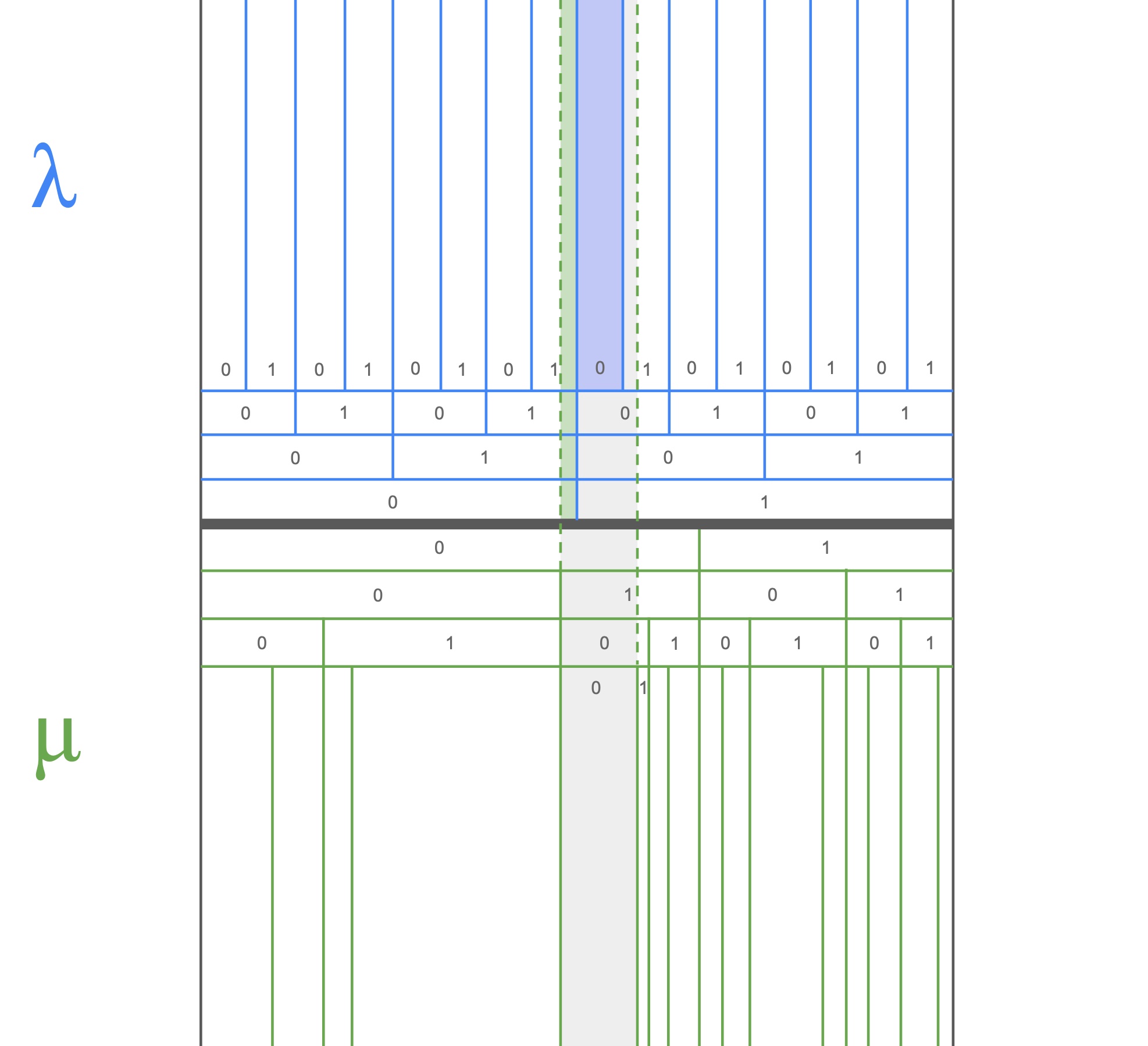
Horizontally we have the real unit interval (isomorphic to the infinite binary sequences). The regions between the blue lines contain all the encoded binary sequences starting with some prefix (under the uniform measure $\l$). The regions between the green lines contain all the decoded binary sequences starting with some prefix (under some measure $\mu$). If we observe that data sequence $\o$ starts with $\o_{1:4}=0100$, then thats equivalent to saying that $\o$ falls within the grey region. An encoding for $\o_{1:4}$ is a region between blue lines that falls entirely within the grey region (because our encoding should uniquely identify $\o_{1:4}$). We can see that the purple region towards the top, identified by the prefix $1000$, is the largest blue region which falls entirely within the grey region (and so has the smallest prefix length). But when we observe more of $\o$, we might discover that $\o$ lies in the green region towards the top, identified by the prefix $01111$. So we would be forced to retroactively switch our prefix from $1000$ to $01111$ as more of $\o$ streams in. A monotonic encoder would not emit anything until enough of $\o$ was read in to uniquely determine the output prefix.