[This is an article, which is something I’ve optimized for readability and transmission of ideas, opposed to notes that are the seed of an idea and something I’ve written quickly.]

This is supplemental material for Liouville's Theorem. Specifically I go through a few examples of phase space transformations, canonical and non-canonical. I also show that we can turn arbitrary configuration space transformations into canonical phase space transformations, a result that will be useful for my discussion about the Bertrand paradox (Liouville's Theorem).

$$
\newcommand{\0}{\mathrm{false}}
\newcommand{\1}{\mathrm{true}}
\newcommand{\mb}{\mathbb}
\newcommand{\mc}{\mathcal}
\newcommand{\mf}{\mathfrak}
\newcommand{\and}{\wedge}
\newcommand{\or}{\vee}
\newcommand{\a}{\alpha}
\newcommand{\b}{\beta}
\newcommand{\s}{\sigma}
\newcommand{\t}{\tau}
\newcommand{\th}{\theta}
\newcommand{\T}{\Theta}
\newcommand{\D}{\Delta}
\newcommand{\d}{\delta}
\newcommand{\dd}{\text{d}}
\newcommand{\pd}{\partial}
\newcommand{\o}{\omega}
\newcommand{\O}{\Omega}
\newcommand{\x}{\xi}
\newcommand{\z}{\zeta}
\newcommand{\r}{\rho}
\newcommand{\fa}{\forall}
\newcommand{\ex}{\exists}
\newcommand{\X}{\mc{X}}
\newcommand{\Y}{\mc{Y}}
\newcommand{\Z}{\mc{Z}}
\newcommand{\P}{\Psi}
\newcommand{\y}{\psi}
\newcommand{\p}{\phi}
\newcommand{\l}{\lambda}
\newcommand{\G}{\Gamma}
\newcommand{\B}{\mb{B}}
\newcommand{\m}{\times}
\newcommand{\E}{\mb{E}}
\newcommand{\R}{\mb{R}}
\newcommand{\H}{\mc{H}}
\newcommand{\L}{\mc{L}}
\newcommand{\e}{\varepsilon}
\newcommand{\set}[1]{\left\{#1\right\}}
\newcommand{\tup}[1]{\left(#1\right)}
\newcommand{\abs}[1]{\left\lvert#1\right\rvert}
\newcommand{\vtup}[1]{\left\langle#1\right\rangle}
\newcommand{\inv}[1]{{#1}^{-1}}
\newcommand{\ceil}[1]{\left\lceil#1\right\rceil}
\newcommand{\dom}[2]{#1_{\mid #2}}
\newcommand{\df}{\overset{\mathrm{def}}{=}}
\newcommand{\up}[1]{^{(#1)}}
\newcommand{\restr}[1]{_{\mid{#1}}}
\newcommand{\dt}{{\D t}}
\newcommand{\Dt}{{\D t}}
\newcommand{\ddT}{{\delta T}}
\newcommand{\Mid}{\,\middle|\,}
\newcommand{\qed}{\ \ \blacksquare}
\newcommand{\diff}[2]{\frac{\dd #1}{\dd #2}}
\newcommand{\diffop}[1]{\frac{\dd}{\dd #1}}
\newcommand{\pdiff}[2]{\frac{\pd #1}{\pd #2}}
\newcommand{\pdiffop}[1]{\frac{\pd}{\pd #1}}
\newcommand{\evalat}[1]{\left. #1 \right|}
$$

Example: Scaling

A simple example to build intuition.

First let’s look at a simple transformation which is not canonical. Define a scaling transformation $Q(q,p)=2q$ and $P(q,p)=2p$. Let’s also consider a specific Hamiltonian, $H(q,p)=\frac{1}{2}p^2$. Then $q(Q,P) = \frac{1}{2}Q$ and $p(Q,P) = \frac{1}{2}P$, and $\tilde{H}(Q,P) = H(q(Q,P),p(Q,P))=\frac{1}{2}\tup{\frac{1}{2}P}^2 = \frac{1}{8}P^2$.

Using the multivariate chain rule we have
$$\begin{aligned}
\diff{Q}{t}&=\pdiff{Q}{q}\diff{q}{t} + \pdiff{Q}{p}\diff{p}{t} \\&= \pdiff{Q}{q}\pdiff{H}{p} - \pdiff{Q}{p}\pdiff{H}{q} \\&= 2p = P
\end{aligned}$$

But $\pdiff{\tilde{H}}{P} = \frac{1}{4}P \neq P = \diff{Q}{t}$, and so we cannot write $\diff{Q}{t} = \pdiff{\tilde{H}}{P}$ in this coordinate system, at least if we want to keep the dynamics of the system the same.

On the other hand, we can make the $Q$-space transformation $Q(q,p)=2q$ canonical by choosing a different $P$-space transformation, specifically $P(q,p)=p/2$. Then $q(Q,P) = \frac{1}{2}Q$ and $p(Q,P) = 2P$, and $\tilde{H}(Q,P) = H(q(Q,P),p(Q,P))=\frac{1}{2}\tup{2P}^2 = 2P^2$.

Then we have

$$\begin{aligned}
\diff{Q}{t}&=\pdiff{Q}{q}\diff{q}{t} + \pdiff{Q}{p}\diff{p}{t} \\&= \pdiff{Q}{q}\pdiff{H}{p} - \pdiff{Q}{p}\pdiff{H}{q} \\&= 2p = 4P
\end{aligned}$$

Thus $\pdiff{\tilde{H}}{P} = 4P = \diff{Q}{t}$, and so Hamilton’s equation is satisfied (clearly $\pdiff{\tilde{H}}{Q}=0=-\diff{P}{t}$).

(This transformation is canonical for all Hamiltonians on 2D phase space)

Hamiltonian Specific Canonical

It is important to clarify the difference between a transformation being canonical for a particular Hamiltonian vs canonical for all Hamiltonians. The derivation in Liouville's Theorem is not specific to any Hamiltonian, and gives us conditions for canonical transformations that are Hamiltonian agnostic.

Let’s take a look at a transformation that is canonical for some but not all Hamiltonians. The following system is a 1D harmonic oscillator (2D phase space). We will perform a Cartesian to polar transformation on phase space. Recall from calculus that Cartesian to polar coordinates has a non-unit Jacobian: $\pdiff{(Q,P)}{(q,p)}=P$ and so $\tilde{\r}(Q,P,t)=P\r(q(Q,P),p(Q,P),t)$ for any density $\r$. Yet in this particular example, we will find that Hamilton’s equations hold in the new coordinate system.

Consider the Hamiltonian $H = \frac{1}{2}\tup{p^2+q^2}$. This is a harmonic oscillator with spring mass $m=1$ and spring constant $k=1$.

To solve the system, use Hamilton’s equations,

$$
\diff{q}{t} = \pdiff{H}{p} = p\,,
$$

$$
\diff{p}{t} = -\pdiff{H}{q} = -q\,.
$$

Solving the PDE system, we get

$$
q(t) = q_0 \cos(t)+p_0 \sin(t)\,,
$$

$$
p(t) = -q_0 \sin(t)+p_0 \cos(t)\,,
$$

where $(q(0),p(0))=(q_0,p_0)$. Basically, the trajectories of this system are circles in phase space centered at the origin. For a given initial condition $(q_0,p_0)$, the trajectory of the system is the circle passing through that point.

Let’s transform to polar coordinates: $Q(q,p)=\tan^{-1}\tup{\frac{p}{q}}$ and $P(q,p)=\sqrt{q^2+p^2}$, giving us the inverse transformation $q(Q,P)=P\cos Q$ and $p(Q,P)=P\sin Q$.

In the transformed coordinate system, $\tilde{H}=\frac{1}{2}\tup{\tup{P\cos Q}^2+\tup{P\sin Q}^2}=\frac{1}{2}P^2$. If we blindly apply Hamilton’s equations in the transformed coordinates we get

$$
\diff{Q}{t} = \pdiff{\tilde{H}}{P} = P\,,
$$

$$
\diff{P}{t} = -\pdiff{\tilde{H}}{Q} = 0\,.
$$

This Hamiltonian corresponds to a free particle at constant momentum. Solutions are $P(t)=P_0$ and $Q(t)=Q_0+P_0t$. These are circular paths in the original coordinate system, and so we have the same trajectories transformed.

As mentioned above transforming 2D phase space to polar coordinates is not measure preserving and in general not a canonical transformation for all Hamiltonians. But for this particular Hamiltonian, our trajectories do not change their distance from the origin, i.e. radius (they trace out circles). The Cartesian to polar transformation is not measure preserving as the radius coordinate changes, but is measure preserving as the angle changes. This transformation preserves rotational symmetry, i.e. density is preserved along circular paths, and our Hamiltonian produces circular paths.

An interesting question to consider: Do all the symmetries of a given Hamiltonian generate transformations canonical to that Hamiltonian? Then it would make sense that if one Hamiltonian obeys a symmetry and another doesn’t, then they wouldn’t share the same canonical transformations. Furthermore, we can recast Liouville’s theorem as stating that for Hamiltonians obeying time-translation symmetry (which are the Hamiltonians conserving energy), time-translations are canonical transformations.

Arbitrary Configuration-Space Transformations

A surprising result is that for all configuration space transformations $\vec{Q}(\vec{q})$, there is a momentum space transformation such that the combined phase space transformation is canonical. My derivation below follows No-Nonsense Classical Mechanics section 7.3.2.

Suppose we are given some configuration space transformation $\vec{Q}(\vec{q})$ which does not depend on the conjugate momenta $\vec{p}$. We can derive the $\vec{P}(\vec{q}, \vec{p})$ needed to make $\vtup{\vec{Q},\vec{P}}(\vec{q}, \vec{p})$ a canonical transformation.

In the Lagrangian formulation of classical mechanics, momentum is defined as $p_i \df \pdiff{\L(\vec{q},\dot{\vec{q}})}{\dot{q_i}}$ where $\dot{q_i} = \diff{q_i}{t}$. The Lagrangian is valid (Euler-Lagrangian equations hold) for all choice of configuration coordinates. Then $P_i \df \pdiff{\L(\vec{q}(\vec{Q}),\dot{\vec{q}}(\vec{Q},\dot{\vec{Q}}))}{\dot{Q_i}}$ where $\vec{q}(\vec{Q})$ is the inverse coordinate transformation and $\dot{q}_i(\vec{Q},\dot{\vec{Q}})=\diffop{t}\left[q_i(\vec{Q})\right]=\sum_{j=1}^n\pdiff{q_i}{Q_j}\diff{Q_j}{t}=\sum_{j=1}^n\pdiff{q_i}{Q_j}\ \dot{Q}_j$.

Then

$$\begin{aligned}
P_i &= \pdiff{\L(\vec{q}(\vec{Q}),\dot{\vec{q}}(\vec{Q},\dot{\vec{Q}}))}{\dot{Q}_i} \\
&= \sum_{j=1}^n \pdiff{\L(\vec{q},\dot{q}_j)}{\dot{q}_j} \pdiff{\dot{q}_j}{\dot{Q}_i} \\
&= \sum_{j=1}^n p_j \pdiff{q_j}{Q_i}\,,
\end{aligned}$$

since $p_j = \pdiff{\L(\vec{q},\dot{q}_j)}{\dot{q}_j}$ and $\pdiff{\dot{q}_j}{\dot{Q}_i}=\pdiffop{\dot{Q}_i}\left[\dot{q}_i(\vec{Q},\dot{\vec{Q}})\right]=\pdiffop{\dot{Q}_i}\left[\sum_{k=1}^n \pdiff{q_j}{Q_k}\dot{Q}_k\right]=\pdiff{q_j}{Q_i}$. Note that $\pdiffop{\dot{Q}_i}\dot{Q}_k = 1$ when $i=k$ and $0$ otherwise, since we take $\dot{Q}_1,\dots,\dot{Q}_n$ to be free variables in the Lagrangian formulation.

In general, the point transformation $\vec{Q}(\vec{q})$ need not be (uniform) measure preserving in configuration space. However, when we consider the combined phase space, the transformation $\vec{Q}(\vec{q})$ and $\vec{P}(\vec{q},\vec{p})=\evalat{\pdiff{\vec{q}}{\vec{Q}}}_{\vec{q}}\cdot\vec{p}$ (where $\pdiff{\vec{q}}{\vec{Q}}$ is the Jacobian matrix evaluated at $\vec{q}$, i.e. $P_i(\vec{q},\vec{p})=\vec{p}\cdot \evalat{\pdiff{\vec{q}}{Q_i}}_{\vec{q}}$ is a dot product) produces a (uniform) measure invariant transformation in phase space.

We can prove this (thus proving Liouville’s theorem) by showing that the Jacobian $\pdiff{(\vec{q},\vec{p})}{(\vec{Q},\vec{P})}=1$ at all locations in phase space.

Example: 2D phase space

Working in 2D phase space is convenient because we can visualize it in full.

Consider the transformation $Q(q)=q^2$.
Inverse: $q(Q) = \sqrt{Q}$.
Then we determine $P(q,p)$,

$$
P(q,p) = p\pdiff{q}{Q} = \frac{p}{2\sqrt{Q}} = \frac{p}{2\sqrt{q^2}} = \frac{p}{2q}
$$

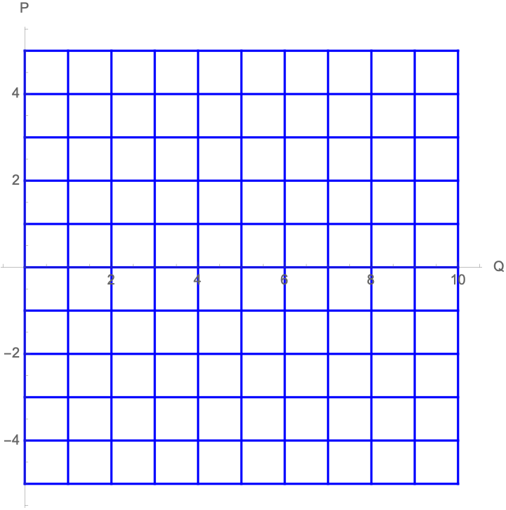
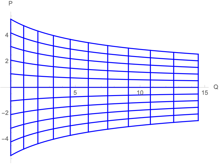
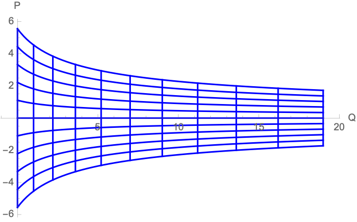
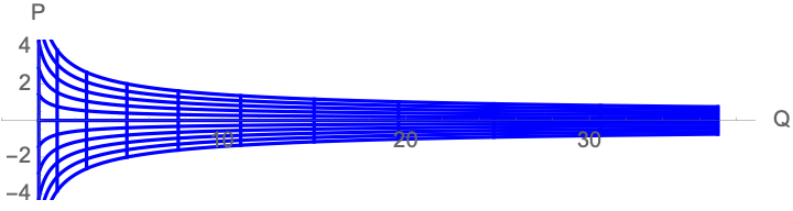
If we want to smoothly interpolate between the old and new coordinates, we can generalize our transformation to $Q(q)=a q^2 + b q$ where $a=\gamma$ and $b=1-\gamma$, where $\gamma$ is our interpolating parameter.
Inverse: $q(Q) = \frac{-b+\sqrt{4 a Q+b^2}}{2 a}$.

$$
P(q,p) = p\pdiff{q}{Q} = \frac{p}{\sqrt{4 a Q+b^2}} = \frac{p}{2 a q + b} = \frac{p}{2 \gamma q + 1-\gamma}
$$

Here we have the Cartesian grid in $(q,p)$ space transformed into $(Q,P)$ space, varying $\gamma$ from 0 towards 1.

Example: Cartesian To Polar Configuration

The result that all configuration space transformations can be made canonical with the right momentum space transformation is surprising because so many configuration space transformations are not measure preserving by themselves. Just above we took the Cartesian to polar transformation as an example of a non-measure preserving transformation. I will go through the derivation of the canonical transformation which does a Cartesian to polar configuration transformation. The reason why this works is that configuration space is an infinitely thin slice of phase space, so all configuration space regions have 0 measure in phase space. Thus there is trivially no need to conserve measure in configuration space alone. The momentum transformation must be such that whatever distortions of measure occur in configuration space are “balanced out” in momentum space.

Consider a system in 4D Cartesian phase space $(x,y,p_x,p_y)$, with $\vec{q}=(x,y)$ and $\vec{p}=(p_x,p_y)$. Let’s give the system the following Hamiltonian, $H=\frac{1}{2m}\tup{p_x^2+p_y^2} + U(x,y)$ where $U$ is some time-independent (constant through time) potential function and $m$ is the mass of the system.

Then by Hamilton’s equations we have

$$
\dot{x}=\pdiff{H}{p_x}=\frac{p_x}{m}\,,\qquad \dot{y}=\pdiff{H}{p_y}=\frac{p_y}{m}\,,
$$

and

$$
\dot{p_x}=-\pdiff{H}{x}=-\pdiff{U(x,y)}{x}\,,\qquad \dot{p_y}=-\pdiff{H}{y}=-\pdiff{U(x,y)}{y}
\,.
$$

These are the standard equations that a Newtonian point particle obeys in the presence of a potential field $U$.

Now transform to polar spatial coordinates: $R(x,y)=\sqrt{x^2+y^2}$ and $\T(x,y)=\tan^{-1}\tup{\frac{y}{x}}$, giving us the inverse transformation $x(R,\T)=R\cos\T$ and $y(R,\T)=R\sin\T$.

We can independently derive the momenta in polar coordinates from Newtonian mechanics: $P_R=m\dot{R}$ and $P_\T=mR^2\dot{\T}$.

Let’s see what momentum transformation we derive using from the constraint that we need a canonical transformation (using the equations above).

$$\begin{aligned}
P_R(x,y,p_x,p_y) &= p_x \pdiff{x}{R}+p_y \pdiff{y}{R} \\
&= p_x \cos\T+p_y \sin\T
\end{aligned}$$

$$\begin{aligned}
P_\T(x,y,p_x,p_y)&=p_x \pdiff{x}{\T}+p_y \pdiff{y}{\T} \\
&= -p_x R\sin\T+p_y R\cos\T
\end{aligned}$$

Solving this system of equations for $p_x,p_y$ we get the inverse transformation for momentum:

$$\begin{aligned}
p_x(R,\T,P_R,P_\T) &= P_R \cos (\T)-\frac{P_\T \sin(\T)}{R} \\
p_y(R,\T,P_R,P_\T) &= P_R \sin (\T)+\frac{P_\T \cos(\T)}{R}
\end{aligned}$$

Plugging in $x(R,\T),y(R,\T),p_x(R,\T,P_R,P_\T),p_y(R,\T,P_R,P_\T)$ to $H(x,y,p_x,p_y)$, we get

$$\begin{aligned}
& H(R,\T,P_R,P_\T) \\
&= \frac{1}{2m}\tup{p_x(R,\T,P_R,P_\T)^2+p_y(R,\T,P_R,P_\T)^2} \\ &\quad\ +\ U(x(R,\T),y(R,\T)) \\
&= \frac{1}{2m}\tup{\tup{P_R \cos (\T)-\frac{P_\T \sin(\T)}{R}}^2+\tup{P_R \sin (\T)+\frac{P_\T \cos(\T)}{R}}^2} \\ &\quad\ +\ U(R\cos\T,R\sin\T)) \\
&= \frac{1}{2m}\tup{P_R^2 + \frac{1}{R^2}P_\T^2} + U(R\cos\T,R\sin\T)
\end{aligned}$$

Then Hamilton’s equations give us

$$
\dot{R}=\pdiff{H}{P_R}=\frac{P_R}{m}\,,\qquad \dot{\T}=\pdiff{H}{P_\T}=\frac{P_\T}{mR^2}\,,
$$

(matching what we expect)

and

$$\begin{aligned}
\dot{P}_R&=-\pdiff{H}{R}\\&=-\pdiff{U(x,y)}{x}\pdiff{x}{R}-\pdiff{U(x,y)}{y}\pdiff{y}{R}\\&=-\pdiff{U(x,y)}{x}\cos\T-\pdiff{U(x,y)}{y}\sin\T\,,
\end{aligned}$$

$$\begin{aligned}
\dot{P}_\T&=-\pdiff{H}{\T}\\&=-\pdiff{U(x,y)}{x}\pdiff{x}{\T}-\pdiff{U(x,y)}{y}\pdiff{y}{\T} \\&= \pdiff{U(x,y)}{x}R\sin\T-\pdiff{U(x,y)}{y}R\cos\T\,.
\end{aligned}$$