
[This is an article, which is something I’ve optimized for readability and transmission of ideas, opposed to notes that are the seed of an idea and something I’ve written quickly.]
All about the bias-variance decomposition as it pertains to machine learning. All you need to know:
$$
\begin{align*}
& \mathbb{E}_D[(f(x; D) - y(x))^2] \qquad\quad\ \textrm{Avg. error}\\
& = (\mathbb{E}_D[f(x; D)] - y(x))^2 \qquad \textrm{Bias}_y(f)^2\\
&\phantom{=}\, + \mathbb{V}_D[f(x; D)] \qquad\qquad\quad\ \, \textrm{Variance}(f)\\
\end{align*}
$$
$$
\newcommand{\Real}{ {\mathbb{R}} }
\newcommand{\E}{ {\mathbb{E}} }
\newcommand{\V}{ {\mathbb{V}} }
\newcommand{\D}{\mathcal{D}}
\newcommand{\Var}{\mathrm{Var}}
\newcommand{\Bias}{\mathrm{Bias}}
\newcommand\Yh{ {\hat{Y}} }
\newcommand{\ep}{ {\boldsymbol{\varepsilon}} }
\newcommand{\s}{\mathbb{S}}
\DeclareMathOperator*{\argmax}{argmax}
\DeclareMathOperator*{\argmin}{argmin}
$$
Preamble
Why am I writing this? In short, because I think there should be an equation somewhere out there that defines the bias-variance decomposition unambiguously and in complete generality.
You’ve likely heard of the bias-variance trade-off. There is not always a trade-off, hence I call it a decomposition. You may think that the trade-off is about trading model flexibility for bias. Probe your understanding and ask yourself, does flexibility always lead to variance? How does flexibility lead to variance? What is varying? The model? The dataset? The variance comes from the model’s interaction with the training data, rather than these things in isolation.
When you picture this trade-off, what comes to mind? A dart-board? A wiggly or rigid function? Those are metaphors - approximations of the concept. Ask yourself, why do the dart throws have bias and variance? How does “wiggliness” contribute to variance? Do some types of wiggliness have less variance than others? These analogies don’t include the source of randomness.
My life is easiest when I am presented with a formal definition. I can then pull nuances out of it, and refer to it to resolve my confusions. My understanding of an idea is as good as its most precise definition. An equation is the bedrock of intuitive understanding.
The power of math is that it is precise, but that precision is lost when an equation has multiple meanings. This ambiguity is only possible when authors take notational shortcuts for visual simplicity and assume the reader can infer the missing information. I prefer a precise equation accompanied by exposition.
So why is this post so long? I could just give the definition (which I did below) and be done with it, but, 1) it’s valuable to unpack the meaning of the equation and explore tricky cases, and, 2) this topic is not so simple, as I discovered while researching this. A truly general definition of the BV-decomposition requires getting abstract… though obscure it’s interesting. However, the special case for ℓ2 loss is all you need to understand and apply this topic.
Context
If you found this post with zero context, the bias-variance (BV) decomposition is a mathematical identity stating that expected prediction errorOn an evaluation/test dataset. of a model equals bias-squared plus variance. The precise meaning of these words is best understood by looking at the equation below.
BV-decomposition is a commonly used idea in machine learning and statistics. Understanding it is essential for communicating with researchers and practitioners. The decomposition (often a trade-off) is used for reasoning about model design. Tons of textbooks and papers give examples of this, e.g. Elements of Statistical Learning, or reinforcement learning literature.
Bias-Variance Decomposition For ℓ2 Loss
This discussion will assume supervised dataI have not seen BV-decomposition for unsupervised models, but my guess is that you can treat it as a supervised problem where $y = p(x)$., e.g. pairs $(x, y)$ where $x$ is an input and $y$ is the observed output. ℓ2Usually noted as $L^2$. Presumably originating from $L^p$-norm. I’m using curly ℓ to avoid confusion when $L$ denotes any loss function. See the Any-Loss section below. lossLoss is machine learning jargon for error function., a.k.a. squared error, is the squared difference between a prediction and the observed output.
The bias-variance decomposition comes from statistics, which considers the error of a parameter estimator. In ML, we are concerned with the error of a model’s prediction (output) and a given target output, which we call the labellabel originates from classification where the model is predicting a nominal value, e.g. category/class. Here I use label to mean to anything that is predicted, and I assume the label is real valued. I just need a word that refers to $y$ in $(x, y)$, including the given/observed and model’s prediction. (a scalar value). The bias-variance decomposition is a mathematical identity stating that expected test loss (prediction error) equals bias-squared plus variance across training datasets. For ℓ2 loss we have,Adapted from the equation in “Neural networks and the bias/variance dilemma”, Geman, S., Bienenstock, E., and Doursat, R. (1992)
$$
\begin{align*}
& \E_D[(f(x; D) - y(x))^2] \qquad\quad\ \textrm{Avg. error}\\
& = (\E_D[f(x; D)] - y(x))^2 \qquad \textrm{Bias}_y(f)^2\\
&\phantom{=}\, + \V_D[f(x; D)] \qquad\qquad\quad\ \, \textrm{Variance}(f)\\
\end{align*}
$$
I am leaving out the derivation of the BV-decomposition, as it can be easily found in a number of sources, including Wikipedia. My purpose here is to clear up common points of confusion.
For completion, here is the definition of $\E$ and $\V$. Let $g:\Real \rightarrow \Real$ be an arbitrary (deterministic and measurable) function over the reals, and $Z$ be an arbitrary random variable over domain $D_Z \subseteq \Real$. Then
$$
\E_Z[g(Z)] = \int_{D_Z} p_Z(z) g(z) dz
$$
is the expected value of $g(Z)$, and
$$
\V_Z[g(Z)] = \E_X[(g(Z) - \E_X[g(Z)])^2]
$$
is the variance of $g(Z)$.
Symbol breakdown
$D$ for dataset
$D$ is a random variable over all possible training datasets. Technically, this equation does not make any assumptions about the nature of the training data, but generally $\{(x_1,y_1),(x_2,y_2), \ldots,(x_n,y_n)\}$ is a sample from $D$, where $(x_i,y_i)$ is an input, $x_i$, with its observed label, $y_i$. Additionally, each $(x_i,y_i)$ is typically assumed to be sampled i.i.d., though that is also not required here either. The dataset size $n$ may be stochastic as well.
The first big point of confusion surrounding BV-decomposition is that the training data comes from a distribution. In practice, you have a fixed dataset, so how does it make sense to take the expectation over all possible training datasets? This equation wants you to imagine that you can draw as many different dataset as you want from the data generating processwhatever physical process produced your current training dataset. That could mean, for example, having photographers go out and take new photos and label the objectsPhotographer + camera + environment + labeler is the physical system that generates the data. You can regard the process as inducing a probability distribution $p(x, y)$. Technically the physical setup would need to be exactly the same each time a photo is taken to sample i.i.d. from $p(x, y)$, but uncorrelated differences in photo taking are fine, e.g. many photographers who have their own styles. I do acknowledge that nothing is truly i.i.d. in reality., or the population census retaken. Redrawing a new training set likely won’t happen in reality, but this is the correct conceptual understanding.
Test on $x$
$x$ is a fixed test input. Our loss $(f(x; D) - y(x))^2$ is measuring test error on $x$. However, we take the expectation of this test error$\E_D[(f(x; D) - y(x))^2]$ over all possible training datasets $D$$x$ may appear in some of them. What $x$ to test on is application dependent, and need not be specified here. It’s important to note that $x$ is held fixed, and not a random variable. This test error equals the model’s bias plus variance on a static input, across all training sets.
Rather than a single test input, you could consider a set of test inputs, $\{x_1,x_2,\ldots,x_m\}$. In which case you are interested in the average loss across the fixed inputs: loss = $\frac{1}{M}\sum_{i=1}^{m} \E_D[(f(x_i; D) - y(x_i))^2]$.
Alternatively you could consider a random variable over all possible test inputs, $X$, and take the expectation test error: loss = $\E_X[\E_D[(f(X; D) - y(X))^2]]$.
The underlying identity is the same in all cases.
Label with $y$
I am assuming a deterministic labeling function $y(x)$ for input $x$. It provides the observed label, a.k.a. ground truth. In practice, the labeling process is also stochastic, and there may not even be a clear truth of the matter. The more general case of the BV-decomposition uses $Y(x)$, where $Y$ is a random variable with conditional distribution, $p_{Y \mid X}(Y \mid X=x)$. $x$ is still a fixed constant here, but could be made a random variable as well if need be.
When $Y(x)$ is stochastic, we get an extra term in the decomposition:
$$
\begin{align}
& \E_{Y(x)}[\E_D[(f(x; D) - Y(x))^2]] \\
& = (\E_D[f(x; D)] - \E_{Y(x)}[Y(x)])^2 \qquad\, \textrm{Bias}_y(f)^2\\
&\phantom{=}\, + \V_D[f(x; D)] \qquad\qquad\qquad\qquad\ \ \, \textrm{Variance}(f)\\
&\phantom{=}\, + \V_{Y(x)}[Y(x)] \qquad\qquad\qquad\qquad\ \ \, \textrm{Variance}(y)\textrm{, i.e. “noise"}
\end{align}
$$
Presumably the human model builder cannot control $\V_{Y(x)}[Y(x)]$, so this is the lower bound on their model’s loss. If bias and variance were reduced to 0, this term would remain.
$f$ is the model + training algo
$f$ is both the model and training algorithm. $f(x; d)$ is a function of input $x$, and a training dataset $d$. $f$ outputs its prediction for $x$, given that it was trained on the dataset. The colon is commonly used in ML to separate model inputs with parameter or training inputs. You can think of $f(d)=f'$ as a outputting another function $f'$ which makes the prediction, $f'(x)$.
This formulation does not make reference to model parameters, and leaves open the possibility of non-parametric models. The BV-decomposition is a universal property, and the process that goes from dataset to predictive model is irrelevant. I am assuming $f$ is deterministic w.r.t. both $x$ and $d$. However, if any of its inputs are random variables, the output is a random variable. So $f(x; D)$ is a random variable, as well as $f(X; d)$.
The second big point of confusion in the BV-decomposition is that the model’s output distribution is the result of applying the model to a training distribution. It does not make sense to talk about the variance of a modelIntrinsic model variance due to stochastic elements like random weight init or stochastic inference is not the primary concern of the BV-decomposition. without reference to its training data, nor are we concerned with the variance of the training data by itself.
In practice, training algorithmse.g. stochastic gradient descent. have stochastic elements, and in some cases predictions can only be samplede.g. generative models like GANs and Boltzmann Machines from the model stochastically. Again, our BV equation can be generalized to include additional sources of randomness by taking the expectation over the additional random variables.
To include noise in the error, you can add $\ep$, a noise random variable, to the arguments of $f$. Loss = $\E_\ep[\E_D[(f(x, \ep; D) - y(x))^2]]$. For training noise, add $\ep$ to the training inputs, i.e. $f(x; D, \ep)$. This difference is purely semantic. Noise is noise.
An Illustration
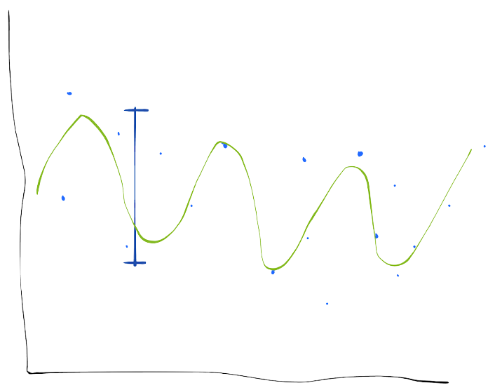
Let’s do a regression problem. We train our model on two different training sets. $x’$ in red is the test data point.
Images made with https://sketch.io/sketchpad/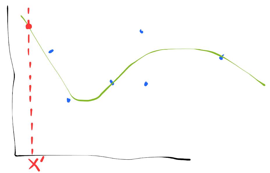
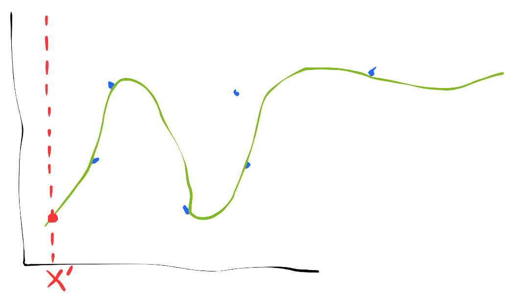
The model’s prediction of test input $x'$ varies greatly between trainings. It is common to say this variance indicates the model is overfitting, which means informally that it’s fitting correlations present in the training set which are not present across datasets. However, overfitting is not an identical concept to variance of a test prediction.
Practitioners would typically say this model has high variance, but that is a jargony shorthand. There is nothing about a model in isolation that has bias or variance. What we really mean is that this particular model applied to this particular training distribution has high variance. This realization affords us two ways to reduce variance:
- Make the size of the training set larger (straight forward to prove that increasing dataset size decreases its variance).
- Make the model less flexible (reduce its capacity)
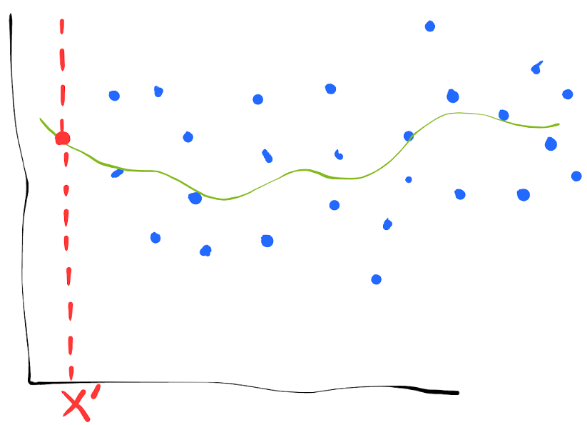
More data, same model flexibility.
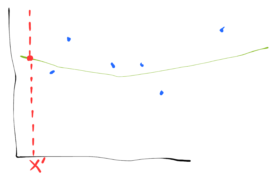
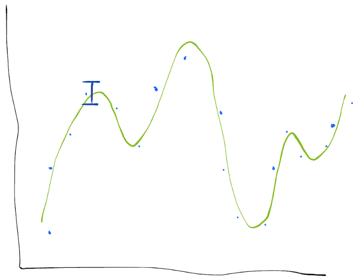
Same data, lower model flexibility.
Note that reducing our model’s flexibility requires making an assumption about our data to reduce the hypothesis space. In this case, perhaps we assumed that our data is drawn from a lower order polynomial. If our constraint/assumption is not well-founded, then the model’s prediction on $x'$ will be systematically wrong, even if the prediction itself does not change much between training sets.
Here is an example of a systematically wrong assumption. We have two training sets as before. The observed label for $x'$ is shown in gray.


This model visually makes a good fit to the training set, but clearly the assumption of linearity is erroneous. Our model’s prediction at $x'$ is wrong by roughly the same amount both times. It has high bias and low variance.
There is only a trade-off from variance to bias when we the experimenters run out of exploitable knowledge about the data. An experimenter with perfect knowledge of the data distribution should be able to build a model that achieves 0 bias and variance (leaving only irreducible noise in the loss). In practice you will eventually reach some limit on your knowledge of the data. Researchers will sometimes try to add bias to their models in ways that reduce its variance. In some cases variance of prediction hurts a lot more than biased prediction, and in other cases you can actually get a slight reduction in overall error in the process of making this trade-off from variance to bias.
Flexibility is broken
Model flexibility is more or less the same concept as model capacity, which is the size of the hypothesis space. A flexible model can fit a more diverse set of functions. A somewhat common belief is that flexibility causes variance, or that flexibility even is variance. Flexibility in my mind is not a well defined concept, but variance is.
What is flexibility? How do you quantify it? How do you compare flexibilities?
A model can be flexible (or inflexible) in many different ways. No matter how flexible a model is, assumptions are made about its hypothesis space. These assumptions are called the inductive biasDefined as a “set of assumptions”. This is qualitative. Not to be confused with statistical bias which is a computable quantity. of the model.
It is important to be clear that model flexibility by itself does not cause bias or variance. Bias and variance are the direct result of how that flexibility (or lack thereof) interacts with the data.
If you know a lot about the structure of your data and you give your model the ability to fit that structure, the variance of your model on that data may be low (picture on the right). You incur variance if that flexibility is not useful (picture on the left).
Bias-Variance Decomposition For Any Loss
Above I defined the bias-variance decomposition for ℓ2 loss. This is the standard presentation, but some will (rightly) question whether this decomposition is universal, meaning that it is true for all loss functions. The preference for ℓ2 loss in statistics is unfortunately somewhat arbitrary, and its popularity is mainly due to its nice math properties. I found a BV-decomposition generalized for all losses in this neat paper by James et al.“Generalizations of the Bias/Variance Decomposition for Prediction Error”, James, G., Hastie, T. (1997), which I will summarize here.
A loss $L : X \times X \rightarrow [0, \infty)$ is a distance function that satisfies,
- $L(x, y) \geq 0$non-negativity
- $L(x, y) = 0 \Longleftrightarrow x = y$identity
- $L(x, y) = L(y, x)$symmetry
- $L$ is convexStronger than requiring triangle inequality.
Note that $L$ operates on a single pair of values, and does not average over a dataset.
James et al. defines the systematic part of random variable $Y$In this section, $Y$ is an underlying data distribution, and $\Yh$ is a model. Both are random variables. I am not showing the dependence of the model on training data and input $X$ for simplicity. In other words, I am not specifying why model $\Yh$ has variance, or even that this model has inputs and is supposed to generalize to a test set. However, everything below still holds with those details added back in. w.r.t. loss $L$,
$$
\s[Y] = \argmin_\theta \E_Y L(Y, \theta)
$$
This generalizes mean. Many common statistics (e.g. mean, median, mode) are the systematic parts for common lossesSource: http://www.johnmyleswhite.com/notebook/2013/03/22/modes-medians-and-means-an-unifying-perspective/.
| $L(y, \hat{y}) =$ | Systematic part |
|---|---|
| $(y - \hat{y})^0$ | Mode |
| $\lvert y - \hat{y} \rvert$ | Median |
| $(y - \hat{y})^2$ | Arithmetic Mean |
| $(\frac{1}{y} - \frac{1}{\hat{y}})^2$ | Harmonic Mean |
| $(\mathrm{ln}(y) - \mathrm{ln}(\hat{y}))^2$ | Geometric Mean |
| $\begin{cases} \tau \cdot (y - \hat{y}) & y - \hat{y} \geq 0 \\ (\tau - 1) \cdot (y - \hat{y}) & \mathrm{otherwise} \end{cases}$ | $\tau$-th Quantile |
Table: $\tau$ is a constant between 0 and 1. $\tau=\frac{1}{2}$ gives the median.
James et al. shards the concepts of bias and variance into additional distinct concepts. For ℓ2 variance, we have the notion of typical distance from some reference point of interest. James et al. points out that there are other ways to define variance which become equivalent under ℓ2 loss, but are not the same in general for other losses.
$$
\begin{align*}
\V_\Yh[\Yh]
& = \E_\Yh(\Yh - \E_\Yh\Yh)^2 \\
& = \E_{Y,\Yh}(Y - \Yh)^2 - \E_Y(Y - \E_\Yh\Yh)^2 \\
\end{align*}
$$
Likewise, bias squared can be written in two different ways.
$$
\begin{align*}
\Bias[Y, \Yh]^2
& = (\E_YY-\E_\Yh\Yh)^2 \\
& = \E_Y(Y-\E_\Yh\Yh)^2 - \E_Y(Y-\E_YY)^2 \\
\end{align*}
$$
When we generalize loss and mean, these alternative ways of writing bias and variance become distinct statistical operations.
The variance effect, $\textrm{VE}[Y, \Yh]$, is the expected change in prediction error when using $\Yh$ instead of $\s[\Yh]$ to predict $Y$. In other words, it measures the effect of predicting with a distribution and all its variability, vs the constant systematic part. This contrasts with intrinsic variance, $\V_\Yh[\Yh]$.
$$
\begin{align*}
\V_\Yh[\Yh] &= \E_\Yh L(\Yh, \s[\Yh]) \\
\textrm{VE}[Y, \Yh] &= \E_{Y,\Yh}[L(Y, \Yh) - L(Y, \s[\Yh])] \\
\end{align*}
$$
The systematic effectNot to be confused with systematic part. Not the terminology I would have gone with., $\textrm{SE}[Y, \Yh]$, is the expected change in prediction error when using $\s[\Yh]$ instead of $\s[Y]$ to predict $Y$. In other words, it measures the effect of predicting with the systematic part of the model, vs the systematic part of the data distribution. This contrasts with intrinsic bias squared, $\Bias[Y, \Yh]^2$.
$$
\begin{align*}
\Bias[Y, \Yh]^2 &= L(\s[Y], \s[\Yh]) \\
\textrm{SE}[Y, \Yh] &= \E_Y[L(Y, \s[\Yh]) - L(Y, \s[Y])] \\
\end{align*}
$$
We may now state the generalized decomposition in terms of systematic and variance effect:
$$
\E_{Y,\Yh}L(Y, \Yh) = \textrm{SE}[Y, \Yh] + \textrm{VE}[Y, \Yh] + \V_Y[Y]
$$
Plugging in, we get,
$$
\begin{align*}
\E_{Y,\Yh}L(Y, \Yh)
&= \E_Y[L(Y, \s[\Yh]) - L(Y, \s[Y])] \\
&\phantom{=}\, + \E_{Y,\Yh}[L(Y, \Yh) - L(Y, \s[\Yh])] \\
&\phantom{=}\, + \E_YL(Y, \s[Y])
\end{align*}
$$
Check out James et al. for some application examples of the generalized BV-decompositionThere exist more exotic BV-decompositions as well, e.g.\nKL-divergence..
What is variance anyway?
I was taught that variance is exactly equal to its ℓ2 definition. I never questioned this until I had a heated argument with a friend who pointed out that variance was a collection of concepts before it was given a formula. The colloquial term variance is defined as “the fact or quality of being different, divergent, or inconsistent”https://www.google.com/search?q=define+variance. As it turns out, there are many ways to formalize aspects of this word, and one is not necessarily better than the other.
Ultimately, the word variance, when used in the context of statistics, will mean ℓ2 variance by convention. Statistical dispersion is the technical name given to the umbrella of variance formulations. For example, Median Absolute Deviation (MAD) is a not-so-obscure alternative to ℓ2 variance for all you median-lovers out there. Entropy is another one. Though not usually thought of as a measure of variance, entropy measures the spread of a distribution without distance to a reference point, which makes it particularly useful for categorical data.
I think formalizing concepts is a big deal, but I don’t take formalisms as absolute truth. They are more like pieces of code that can be connected together and modified. I am picky when it comes to the API that a math definition uses, i.e. the objects that are abstracted away. I expect my formula to be general purpose, but there is not going to be a definition that captures all possible cases of an idea. My philosophy is to start with good math, and use it to understand the nuances of an idea. Then use intuition and creativity to think about the idea in new ways, and potentially invent a new formalism. The math you started with gives you a foundation for building and a sandbox for playing.
Acknowledgments
I want to thank John Chung, Frazer Kirkman, Ivan Vendrov, and Roman Novak for their valuable discussions and feedback on this post. I give special thanks to Jeremy Nixon who inspired me to research this topic thoroughly and offered insights on the interaction between mathematics and informal ideas in research.