
[This is an article, which is something I’ve optimized for readability and transmission of ideas, opposed to notes that are the seed of an idea and something I’ve written quickly.]
David Chapman’s blog post titled Probability theory does not extend logic has stirred up some controversy. In it, Chapman argues that so-called Bayesian logic, as it currently understood, is limited to propositional logic (0th order logic), but cannot generalize to higher order logics (e.g. predicate logic a.k.a. 1st order logic), and thus cannot be a general foundation for inference from data under uncertainty.
Chapman provides a few counter-examples that supposedly demonstrate that doing Bayesian inference on statements in 1st order logic is incoherent. I think there is a lot of confusion surrounding this point because Chapman does not use proper probability notation. In the following article I show how Chapman’s examples can be properly written and made sense of using random variables. Hopefully this clarifies some things.
It’s a good exercise to see what would happen if you tried to do Bayesian inference on statements in 1st order logic, but I make no endorsements on what you should do. Such constructions, though syntactically valid, are often undecidable (or non-computable), and otherwise intractable to even approximate. It’s also not clear that you gain more power from doing so (see my section on infinite coin tossing).
Admittedly, this article is obnoxiously long. It’s not necessary to read all of it. In summary, I …
- Explain how probability notation is supposed to work.
- Review Bayesian 0th-order logic and explain my understanding of Bayesian probability.
- Go through some examples that hopefully demonstrate natural ways that probability and 1st-order logic can interact.
- (then finally) reinterpret Chapman’s “challenge” problems.
I also posted a shorter version of this on LessWrong.
What is “Bayesian” anyway?
Just to say a bit more about the confusions in this conversation …
For a while I had misunderstood what position Chapman is arguing against (I’m not sure I understand it now). Chapman’s writing is a continuation of the “great conversation” that took place throughout the 20th century, about the interplay between probability, epistemology and AI. Some camps believe that formal logic is the path to AI. An offshoot of that camp believe that formal logic combined with probability is the path to AI. The latter are often called “Bayesians”. If I understand correctly, Chapman is perhaps part of a third camp that believes formal methods alone cannot lead to AI.
In the aforementioned post, Chapman is addressing a particular link in the chain of justifications for the Bayesian camp: that probability extends formal methods in general. I’m not sure I fully get what that means, but the gist of it seems to be that, supposing you wanted to do logic under uncertainty, then there is exactly one formalism that you should use: probability. This has the benefit of simplifying the great epistemological debate in AI to: “The solution is either be our method (the Bayesian method) or something totally unknown.”
In the case of propositional (0-th order) logic, “extending logic to include uncertainty” and “putting a probability distribution over logical propositions” turn out to be equivalent ideas. For higher-order logics (1st-order and above), there does not appear to be such an equivalence. I’ll just point out that Chapman isn’t saying that probabilistic 1st-order logic is impossible, but that it has not been figured out yet. He cites the Stanford Encyclopedia of Philosophy’s entry on logic and probability on this point.
The problem is that I don’t think “Bayesianism” means the same thing today. For instance, those who advocate for Bayesian methods in machine learning, are advocating for Bayesian models of any kind (these days Bayesian neural networks). Formal logic in particular has gone out of vogue (from what I can tell) as a path towards AI (though I think there is still ongoing Bayesian networks research, which could count as Bayesian logic).
For someone like me who sees the Bayesian position in this much broader sense, I don’t know why you would want to formalize mathematics and/or logic inside probability theory. That just sounds like an unnecessary headache. The standard formalizations of mathematics (e.g. Zermelo–Fraenkel set theory (ZF) or type theory) allow you to define probability theory within them (that’s what the Kolmogorov axioms do). Since any formalization of mathematics at least as powerful as ZF set theory is a higher-order logic, that should mean you can freely mix higher order logic and probability. Why do we need to make probability a foundation? We get what we want for free using the standard definitions of things.
The Formalism
$$
\newcommand{\ex}{\exists}
\newcommand{\fa}{\forall}
\newcommand{\es}{\emptyset}
\newcommand{\and}{\wedge}
\newcommand{\or}{\vee}
\newcommand{\xor}{\veebar}
\newcommand{\subs}{\subseteq}
\newcommand{\mc}{\mathcal}
\newcommand{\mf}{\mathfrak}
\newcommand{\mb}{\mathbb}
\newcommand{\bs}{\boldsymbol}
\newcommand{\ol}{\overline}
\newcommand{\abs}[1]{\left\lvert#1\right\rvert}
\newcommand{\N}{\mb{N}}
\newcommand{\B}{\mb{B}}
\newcommand{\Z}{\mb{Z}}
\newcommand{\R}{\mb{R}}
\newcommand{\t}{\tau}
\newcommand{\th}{\theta}
\newcommand{\ep}{\epsilon}
\newcommand{\vep}{\varepsilon}
\newcommand{\set}[1]{\left\{#1\right\}}
\newcommand{\tup}[1]{\left(#1\right)}
\newcommand{\atup}[1]{\left\langle#1\right\rangle}
\newcommand{\r}{\bs}
\newcommand{\bool}{\mathrm{Bool}}
\newcommand{\0}{\mathrm{false}}
\newcommand{\1}{\mathrm{true}}
\newcommand{\Mid}{\,\middle|\,}
\newcommand{\O}{\Omega}
\newcommand{\o}{\omega}
$$
I’m going to use standard measure-theoretic probability (i.e. the Kolmogorov axioms) defined within whatever standard formalization of mathematics you like (e.g. set theory or type theory). I won’t address undecidability. Just know that undecidability can be handled the same way that Solomonoff handles it, i.e. by using semimeasures instead of measures (see Marcus Hutter’s book for an explanation of this). Meaning, probability may sum to less than 1, where the missing probability is placed on statements that are undecidable.
Quick review of probability theory
For an in-depth review of probability theory, see my post: Probability Theory and Its Philosophy.
First, we need a set of possibilities, $\Omega$, called the sample set (or sample space). A random process chooses a particular sample $\omega \in \Omega$. The word “sample” here is not intended to mean a collection of datapoints. I prefer to think of $\o$ as a possible world state.
The triple $(\Omega, E, P)$ (or $(\Omega, E, \mu)$) is called a probability space, which is a type of measure space.
$P$ (or sometimes $\mu$) is a measure, which is a function mapping subsets of $\Omega$ to real numbers between 0 and 1 (inclusive).
$E \subseteq 2^\Omega$ is the event set, i.e. set of measurable sets of samples $\omega$. By default assume $E = 2^\Omega$. Don’t worry about this detail.
Then $P: E \to [0,1]$.
A probability measure is different from a probability mass (or density) function. $P$ is a function of sets. A probability mass function, e.g. $F : \Omega \to [0,1]$, is a function of samples.
$P(\set{\omega_1, \omega_2, \omega_3})$ is valid.
$P(\set{\omega})$ is valid.
$P(\omega)$ is invalid. You should write $F(\omega)$ where $F$ is the probability mass function for $P$, i.e. $F(\omega) = P(\set{\omega})$.
Having two kinds of probability functions is annoying, so we can pull some notational tricks. For example, leave out function call parentheses:
$$
P\set{\omega} = P(\set{\omega})\,.
$$
Another trick is to use random variables:
$$
P(\r{X} = x)
$$
expands out to
$$
P\set{\omega \in \Omega \mid \r{X}(\omega) = x}
$$
where the contents of $P(\ldots)$ are a boolean expression (i.e. a logical proposition), and bold variables become functions of $\omega$ in the set-constructor version.
The bold variables are called random variables, which are (measurable; but don’t worry about this) functions from $\Omega$ to any type you wish (whatever is useful for expressing the idea you want to convey).
We can have the identity random variable $\r{\o} : \Omega \to \Omega : \omega \mapsto \omega$, and write
$$
P(\r{\o} = \omega^*) = P\set{\omega \in\Omega \mid \r{\o} = \omega^*}
$$
Note that the expression $P(\r{\o})$ is invalid because the contents of $P(\ldots)$ are not a logical proposition. The contents must either be a subset of $\Omega$ (specifically an element of $E$ called an event), or a boolean expression that can be used to construct a subset of $\Omega$ (event in $E$).
Note that while I am bolding random variables to remove ambiguity, this is not notationally required, so long as its clear which symbols in $P(\ldots)$ are the random variables.
General random variable notation
My definition may be a bit idiosyncratic. For any boolean-valued random variable, i.e. a (measurable) function $\r{Z}: \O \to \bool$, we define
$$
P(\r{Z}) := P\set{\o\in\O \mid \r{Z}(\o)}
$$
which is the $P$-measure of the set of all $\o\in\O$ s.t. $\r{Z}(\o)$ is true. $\set{\o\in\O \mid \mathrm{predicate}(\o)}$ is called set-builder notation. Here, our boolean-valued function $\r{Z}$ acts as a logical predicate.
Combining that with the shorthand convention that arbitrary mathematical operations on random variables produces random variables, and we get the usual notation that
$$
P(\mathrm{expr}(\r{X}_1, \r{X}_2, \r{X}_3, \ldots)) = P\set{\omega \in \Omega \mid \mathrm{expr}(\r{X}_1(\omega), \r{X}_2(\omega), \r{X}_3(\omega), \ldots)}\,,
$$
where $\r{X}_1, \r{X}_2, \r{X}_3, \ldots$ are random variables of any type (not necessarily Boolean-valued) and $\mathrm{expr}(\r{X}_1, \r{X}_2, \r{X}_3, \ldots)$ is any boolean-valued expression involving arithemtic operators, functions, and logical expressions.
For example, if $\r{X}_1, \r{X}_2$ are real-valued, then $\r{X}_1 + \r{X}_2 = 5$ is a shorthand for the boolean-valued function $\o \mapsto (\r{X}_1(\o) + \r{X}_2(\o) = 5)$. Another example is $\r{X}_1^2 > 4 \and \sin(\r{X}_2) \in [0,1]$, which is a shorthand for the boolean-valued function $\o\mapsto(\r{X}_1(\o)^2 > 4 \and \sin(\r{X}_2(\o)) \in [0,1])$. In general, anything that you can symbolically do to regular variables $x_1, x_2, x_3 \ldots$ you can do to random variables $\r{X}_1, \r{X}_2, \r{X}_3, \ldots$.
Conditional probability
For sets $A,B\subseteq\O$ (called events) we define
$$
P(A \mid B) := P(A\cap B)/P(B)\,.
$$
Random variables inside this conditional notation expand out into sets just as before. Thus, for boolean-value random variables $\r{Y}, \r{Z}$, we have
$$
\begin{aligned}
&P(\r{Z} \mid \r{Y}) \\
&\quad= P(\set{\o\in\O\mid\r{Z}(\o)}\mid\set{\o\in\O\mid\r{Y}(\o)}) \\
&\quad= P(\set{\o\in\O\mid\r{Z}(\o)}\cap\set{\o\in\O\mid\r{Y}(\o)})/P\set{\o\in\O\mid\r{Y}(\o)} \\
&\quad= P\set{\o\in\O\mid\r{Z}(\o) \and \r{Y}(\o)}/P\set{\o\in\O\mid\r{Y}(\o)} \\
&\quad= P((\r{Z}\and\r{Y})^{-1}(\1))/P(\r{Y}^{-1}(\1))\,.
\end{aligned}
$$
where $\r{Y}^{-1}(\1)$ is the preimage of $\r{Y}$ on $\1$, i.e. the set of all inputs $\o\in\O$ s.t. $\r{Y}(\o)$ is true. Likewise, $(\r{Z}\and\r{Y})^{-1}(\1)$ is the preimage of the function $\r{Z}\and\r{Y}$ on $\1$.
The intuitive way to think about the conditional probability operator, is that it is a domain-restriction followed by a rescaling. $P(\cdot)$ is adding up probability over the domain $\O$, while $P(\cdot \mid \r{Y})$ is adding up rescaled-probability over the domain $\r{Y}^{-1}(\1)$. The probabilities are rescaled s.t. they sum to 1 over the restricted domain $\r{Y}^{-1}(\1)$.
In general, conditioning on knowns/observations is just a matter of restricting your possibility space to the subspace where the knowns/observations hold true. Pretty straightforward. Later on, we will encounter some gnarly conditional probabilities, so it is very helpful to keep in mind that this operation really denotes a simple idea.
Quantifiers inside probability
There is no reason why we cannot build a boolean-valued function involving logical quantifiers. Just by using the standard formulation of probability and random variables, we get probabilities of quantifiers for free.
Before getting into the interpretation of such constructions, i.e. “what does it mean to take the probability of a quantifier and why would you want to?”, let’s just go through the notational machinery to see what happens if we blindly obey our definitions.
1st order logic (aka predicate logic) is logic with quantifiers, type sets, and predicates. Here, a boolean-valued random variable (function on samples $\o$) acts like a predicate.
The standard quantifiers are “for-all” and “there-exists”. For example, $\fa a \in A : f(a)$ is a logical proposition (it is a statement that is not a function of any free variable) which says that for all elements $a$ in $A$, $f(a)$ is true, where $f : A \to \bool$ is some predicate, i.e. boolean-valued function on set $A$. We could also make a predicate containing a quantifier, e.g. $g : B \to\bool : b \mapsto \fa a \in A: f(a,b)$ for some multi-agument predicate $f : A\times B \to \bool$ (I’m using “mapsto” function notation). In this way we can nest predicates or quantifiers.
If we wanted to measure the probability that $\fa x \in X : f(x)$ is true, we need to convert this proposition (i.e. not a function) into a function on sample space $\O$. There are two avenues for doing so, you can make $X$ a function on $\O$ or make $f$ a function on $\O$ (or both).
So we have
$$
P(\fa x \in \r{X} : \r{f}(x)) = P\{\omega \in \Omega \mid (\fa x \in \r{X}(\omega) : \r{f}(\omega)(x))\}\,,
$$
$$
P(\ex x \in \r{X} : \r{f}(x)) = P\{\omega \in \Omega \mid (\ex x \in \r{X}(\omega) : \r{f}(\omega)(x))\}\,.
$$
Here, $\r{X}$ is a set-valued random variable, and $\r{f}$ is a function-valued random variable. Meaning, $\r{X}:\O \to U$ where $U$ is a set of sets (or perhaps the powerset of some set), and $\r{f} : \Omega \to \mathrm{Predicates}$ where $\mathrm{Predicates}$ is a set of functions with signatures $X' \to \bool$ for all $X' \in U$. Assume that probability measure $P$ is chosen such that for all $\omega \in \Omega$, $\r{f}(\omega)$ is a valid predicate for domain $\r{X}(\omega)$. This allows us to side-step type issues.
A brief prelude on the interpretation of what we’ve just created: $\r{X}$ is the domain of quantification. If the domain is a random variable, we can take that to mean we have uncertainty about what domain to quantify over. If a predicate is a random variable, we can take that to mean we have uncertainty about what predicate to use. I call both of these kinds of uncertainties definitional uncertainty. More on that later.
On structured possibility spaces
In general, I want to be able to suppose that $\o\in\O$ is a structured type without having to go into what that structure might be every time. By “structured type”, I mean it is composed of other types just like a struct in programming. Running with the programming analogy, suppose $\O$ is the set of all instances of:
$$
\begin{aligned}
&\texttt{struct Primitives \{ } \\
&\qquad X : 2^\Z, \\
&\qquad f : \mathrm{Predicates} \\
&\qquad v : \bool^n, \\
&\qquad \mathrm{Noise} : \set{0,1}^m,\\
&\texttt{\}}
\end{aligned}
$$
where $2^\Z$ is the powerset (set of all subsets) of $\Z$ (if we include infinite subsets we are straying away from the computing analogy, but hey, this math!). This means that any given $\o\in\O$ specifies a domain $X$, a predicate $f$, a vector of primitive propositions $v$, and a noise vector $\mathrm{Noise}$.
Then it is straightforward to define the following random variables:
- $\r{X} : \O \to 2^\Z$ is the domain of quantification, e.g. $\fa x \in\r{X} : \r{f}(x)$.
- $\r{f} : \O \to \mathrm{Predicates}$ is a predicate.
- $\r{v} : \O \to \bool^n$ is a vector of Booleans which we can take to be primitive propositions.
- $\r{\mathrm{Noise}} : \O \to \set{0,1}^m$ is a vector of noise.
So when I suppose there is a possibility space $\O$ without saying anything about its structure, and I proceed to define a bunch of random variables with very different types, e.g. $\r{X} : \O \to 2^\Z, \r{f} : \O \to \mathrm{Predicates}, \r{v} : \O \to \bool^n, \r{\mathrm{Noise}} : \O \to \set{0,1}^m$, you can see how $\o\in\O$ might be defined such that the random variables are mutually compatible with one-another, i.e. the same $\o$ can simultaneously encode wildly different data-types.
Review of Bayesian Propositional (0-th order) Logic
$$
\newcommand{\P}{\mc{P}}
\newcommand{\Q}{\mc{Q}}
$$
It is instructive to see what so-called Bayesian propositional logic typically refers to. I’ll go through it using the same notation and perspective I’ve introduced above.
In propositional logic you start with a set of primitive propositions, which I’ll denote here as $\P_1, \P_2, \P_3, \ldots$ (not to be confused with probability measure $P$). Derived propositions are formed by logical operations on primitive propositions, e.g. $\Q := (\P_1 \and \P_2) \or \neg \P_3$. We wish to discover what universe we actually inhabit. That is to say, what are the actual Boolean values of all the primitive propositions $\P_1, \P_2, \P_3, \ldots$. For example, if you observe $\P_2 = \1,\ \P_3 = \1$ and $\Q = \0$, then we can uniquely determine that $\P_1 = \0$ (you can verify this yourself by writing out the truth table).
The probabilistic version of propositional logic puts a probability distribution over the primitives $\P_1, \P_2, \P_3, \ldots$, which induces a distribution over the derived propositions such as $\Q$.
Let $P$ be a probability measure on $\O = \bool^n$, the set of all $n$-vectors of truth values for $\P_1, \ldots, \P_n$. Then, for example, the probability that $\P_1 \and \neg\P_2 \and \neg\P_3 \and \ldots \and \P_n$ is true is the probability measure of the boolean vector
$$
P\set{\atup{\1,\0,\0,\ldots,\1}}\,.
$$
We can make this notationally easier by defining our propositions as random variables, i.e. $\r{\P}_i : \bool^n \to \bool : \atup{b_1, \ldots, b_n} \mapsto b_i$ for $i \in \set{1,\ldots,n}$ returns the $i$-th boolean value. Then we can write
$$
\begin{aligned}
&P(\r{\P}_1 \and \neg\r{\P}_2 \and \neg\r{\P}_3 \and \ldots \and \r{\P}_n) \\
&\quad= P\set{\o\in\bool^n \mid \r{\P}_1(\o) \and \neg\r{\P}_2(\o) \and \neg\r{\P}_3(\o) \and \ldots \and \r{\P}_n(\o)} \\
&\quad= P\set{\atup{\1,\0,\0,\ldots,\1}}\,.
\end{aligned}
$$
We can also compute marginal probabilities, e.g. $P(\r{\P}_1) = P\set{\o\in\bool^n \mid \r{\P}_1(\o)} = P\set{\atup{\1, \\\_, \\\_, \ldots} \in \bool^n}$ which is the total probability across all Boolean vectors where the first entry is true.
We can straightforwardly compute the probability of more complex expressions, e.g.
$$
P((\r{\P}_1 \and \r{\P}_2) \or \neg \r{\P}_3) = P\set{\o\in\bool^n \mid (\r{\P}_1(\o) \and \r{\P}_2(\o)) \or \neg \r{\P}_3(\o)}\,.
$$
which is the sum of probability of all Boolean $n$-vectors s.t. the proposition $\Q$ from above is true. If we define a derived random variable $\r{\Q} = (\r{\P}_1 \and \r{\P}_2) \or \neg \r{\P}_3$, then we can simply write,
$$
P(\r{\Q}) = P((\r{\P}_1 \and \r{\P}_2) \or \neg \r{\P}_3) = \ldots
$$
Using random variables, we get probabilistic propositional logic “for free”, in the sense that really the standard axioms of probability and mathematics allow us to essentially combine probability with logical statements in the way we’d like.
We can also infer unknowns from knowns. Above I gave the example of uniquely determining $\P_1=\0$ from $\P_2=\1,\P_3=\1,\Q=\0$. Suppose instead we want to infer $\Q$ only given $\P_1=\1,\P_2=\0$. Clearly $\Q$ is underdetermined without knowing $\P_3$, but we can calculate the probability of $\Q=\1$ given $\P_1=\1,\P_2=\0$,
$$
\begin{aligned}
&P(\r{\Q} \mid \r{\P}_1 \and \neg\r{\P}_2) \\
&\quad= P\set{\o\in\bool^n \mid \r{\Q}(\o) \and \r{\P}_1(\o) \and \neg\r{\P}_2(\o)} / \mc{Z} \\
&\quad= P\set{\o\in\bool^n \mid ((\r{\P}_1(\o) \and \r{\P}_2(\o)) \or \neg \r{\P}_3(\o)) \and \r{\P}_1(\o) \and \neg\r{\P}_2(\o)} / \mc{Z} \\
&\quad= P\set{\o\in\bool^n \mid \r{\P}_1(\o) \and \neg\r{\P}_2(\o) \and \neg\r{\P}_3(\o)} / \mc{Z}
\end{aligned}
$$
where $\mc{Z} = P\set{\o\in\bool^n \mid \r{\P}_1(\o) \and \neg\r{\P}_2(\o)}$ is the normalizing constant. (Going forward I will denote $\mc{Z}$ as the normalizing constant without expanding it out, to keep things from getting cluttered, and to show that it represents a simple idea: that the probabilities need to be rescaled to the new domain being conditioned on.)
Depending on your choice of $P$, the probability $P(\r{\Q} \mid \r{\P}_1 \and \neg\r{\P}_2)$ may be anywhere between 0 and 1, indicating that $\Q$ is underdetermined for the given knowns.
If you wanted to model stochastic propositions, e.g. $\Q$’s dependency on $\P_1,\P_2,\P_3$ is stochastic, you can just designate part of the sample $\o$ as noise (typically unobserved) and have $\Q$ depend on it. For example, let $\r{N} : \O \to \bool$ be a noise random variable. Define $\r{\Q}' = \r{Q} \xor \r{N}$ where $\xor$ denotes exclusive “or”. Then $\r{N}$ randomly flips $\r{Q}$. The probability that $\r{Q}'$ is true given the truth values of $\P_1,\P_2,\P_3$ is given by,
$$
P(\r{Q}' \mid \r{\P}_1 = b_1 \and \r{\P}_2 = b_2 \and \r{\P}_3 = b_3)\,.
$$
Your choice of $P$ determines the distribution on $\r{N}$, i.e. how noisy $\r{Q}'$ is (low chance of bit flipping means $\r{Q}'$ is less noisy).
Note that I assumed we have finitely many primitive propositions. We generally wouldn’t have infinitely many, because if we think of primitive propositions as axioms, that would be like having an infinite number of axioms which is generally more powerful than finitely many axioms. 1-st order logic can be thought of as a kind of logic that allows for infinitely many propositions, e.g. predicate $f$ applied to $\N$ generates the propositions $p(0), p(1), p(2), \ldots$. Later on, I will cover tricky issues that come about when $\O$ is an infinite Cartesian product.
Philosophy of Bayesian Probability
The core perspective driving everything that will follow, is that the sample set $\O$ respresents our possible universes (or possible worlds, depending on your preferred aesthetic), and we are trying to figure out which $\o\in\O$ is actually the case by conditioning on observations to narrow down $\O$ (conditioning on givens is a domain restriction). We will do so by starting with a probability measure $P$ on $\O$ and then progressively narrow down the possibility space by conditioning on observations (i.e. givens). Note that $P$ and $\O$ are never modified during the course of “learning”, i.e. observing data and updating beliefs. (I sympathize if this is counterintuitive. It reminds me of anamnesis).
The term “Bayesian” doesn’t have a precise meaning, so I will give it one for the purposes of this article. When I say I am being Bayesian, or I am using Bayeisan probability, that indicates that I have a possibility space $\O$ and a probability measure $P$ on $\O$ called the prior. “Bayesian” is in contrast to a framework where there is no probability measure on $\O$, which requires a different way of updating on observations. I’m NOT saying that one framework is better than the other. The problem posed is how Bayesian probability can incorporate quantifiers in 1st order logic, and I am meeting that challenge.
It is true that this Bayesian framework implies a particular interpretation on what probability does. The conventional interpretation of “the probability of x” is that it quantifies the fraction of outcomes where “x happens” out of a total number of independent trials. In contrast, I am not supposing that we have repeated trials of anything. I am instead supposing that one particular reality $\o$ is the case out of a space of possible realities $\O$, for all time. Nothing needs to be repeating (though it can if you choose the right $\O$ and $P$). In that sense, the Bayesian framework is different from the frequentist framework of independent repeating trials (again “frequentist” has no precise definition so I’m giving it one here, and I am not saying that one is better than the other).
At the same time, the Bayesian framework is agnostic to whether probability is objective or subjective. The math is the same either way. There are actually many different notions of Bayesian probability. Conventionally, $\O$ and $P$ are regarded as an agent’s model rather than literally representing the environment. $P$ might reflect what an agent aught to rationally believe (objective Bayesian) or what an agent chooses to believe (subjective Bayesian). Either way, $P\set{\o}$ (or $P(E)$ for some event $E\subset\O$) can be interpreted as a representation of how plausible the agent believes $\o$ is.
Motivating examples
Before addressing Chapman’s Bayesian 1st order logic examples, I want to demonstrate that sensible use cases for combining Bayesian probability and 1st order logic. I’ll go through two motivating examples, which also serve as intuition pumps for when we tackle Chapman’s examples later.
Motivating Example 1: Unicorns
What is the probability that there exists a unicorn?
What is the probability that all unicorns have one horn?
These may seem like absurd questions, but they can be made rigorous.
Suppose I model reality in the way we did above. I have a space of primitive states $\Omega$, and derived objects which are functions on $\Omega$.
An extreme example would be that I have some kind of model of physics, and the state of the universe $\omega \in \Omega$ is a space-time block of matter-energy. I also have a unicorn recognition function $\mathrm{IsUnicorn} : \zeta \to \bool$ which takes as input a subset of matter-energy in some space-time region of $\omega$, denoted as $\zeta$, and returns whether $\zeta$ is a unicorn. We can think of $\zeta$ as a substate of $\omega$, since $\zeta$ is some piece of it. Specifically, $\zeta = \mathrm{Slice}\_{R}(\omega)$ where $R$ is a spacetime region of $\omega$. Since $\mathrm{Slice}\_{R}$ is a function of state, it is also a random variable (assuming it is measurable). If we construct the set of all slices obtained at all spacetime regions $Z(\omega) = \set{\mathrm{Slice}_{R}(\omega)}_R$, then this too is a random variable. Then we can query
$$
\ex \zeta \in Z(\omega) : \mathrm{IsUnicorn}(\zeta)\,,
$$
which asks if there exists a slice of $\omega$ that is a unicorn, in effect, does there exist a unicorn (given that the universe has state $\omega$).
If we put a prior (probability measure) $P$ over state space $\Omega$ (reflecting our lack of knowledge about what state the universe is actually in), then we can write
$$
\begin{aligned}
& P(\ex \zeta \in \bs{Z} : \mathrm{IsUnicorn}(\zeta)) \\
&\quad = P\set{\omega \in \Omega \mid \ex \zeta \in \bs{Z}(\omega) : \mathrm{IsUnicorn}(\zeta)}\,.
\end{aligned}
$$
I’m using bold to denote what is a random variable, though this is not notationally necessary.
Note that this probability is not a property of the universe, but a property of our model of the universe (the sample space $\Omega$ and probability measure $P$).
Definitional uncertainty
Another source of uncertainty about whether unicorns exist, is from definitional uncertainty. I might be unsure about what constitutes a unicorn. For example, is any horse with a horn considered a unicorn? If my model includes horses, I should be able to compute the probability that there exist horses with horns. Can a unicorn have two horns? If I entered a VR simulation and encountered a unicorn, does that count as unicorns existing? Rather than commit arbitrarily to a particular definition, I can extend Bayesian evenhandedness to choices of definition, and more broadly, choices of ontology (how I conceptually divide up experience), by creating a mixture over the possibilities.
For example, suppose I am unsure about whether to allow unicorns to have two horns (as well as one). Let’s suppose I have two versions of my function from above: $\mathrm{IsUnicorn}_1(\zeta)$ is strict and only allows unicorns to have exactly one horn, while $\mathrm{IsUnicorn}_2(\zeta)$ is lax and allows unicorns to have one or two horns. Then, if I choose $\mathrm{IsUnicorn}_1$ as my definition for unicorn, all unicorns have one horn. Otherwise, if I choose $\mathrm{IsUnicorn}_2$ then not all unicorns necessarily have one horn. Suppose we also have an auxillary function $\mathrm{NumHorns}(\zeta) \to \N$, then we can formalize the query:
$$
\fa \zeta \in Z(\omega) : (\mathrm{IsUnicorn}_n(\zeta) \implies \mathrm{NumHorns}(\zeta)=1)\,,
$$
for $\omega \in \Omega$ and $n \in \set{1,2}$.
Now if we consider $n$ to be part of our primitive state and put a prior $P$ over the combined state $(\omega,n) \in \Omega\times\set{1,2}$, we can write
$$
\begin{aligned}
& P(\fa \zeta \in \bs{Z} : (\bs{\mathrm{IsUnicorn}}(\zeta) \implies \mathrm{NumHorns}(\zeta)=1)) \\
&\quad = P\set{(\omega,n) \in \Omega\times\set{1,2} \mid \fa \zeta \in \bs{Z}(\omega) : (\bs{\mathrm{IsUnicorn}}_n(\zeta) \implies \mathrm{NumHorns}(\zeta)=1)}\,.
\end{aligned}
$$
This probability is strictly between 0 and 1 if I put non-zero probability on $\mathrm{IsUnicorn}_1$ and $\mathrm{IsUnicorn}_2$, since the proposition is true for the former and false for the latter.
In a sense, you can think of an agent with such a prior as supposing two different kinds of universes, each with state-uncertainty. In one universe unicorns have exactly one horn. In the other universe, they can have one or two horns. At this point, it is more sensible to consider $P$ and $\O$ to be the agent’s model, rather than some physically meaningful possibility space (or perhaps a combination of both).
Note that definitional uncertainty is different from logical uncertainty, which is uncertainty about necessary logical implications from given axioms due to computational limitations. That is to say, logical uncertainty is uncertainty about what is logically true within a formal system (given infinite compute) vs uncertainty about what formalisms are to be used (informally, uncertainty about how to slice up your perceived reality into definitions and concepts).
Motivating Example 2: Rigged Poker
Suppose I’m playing poker, and I have reason to suspect the dealer has rigged the game by removing cards from the deck. If the set of all cards in a full deck is $\mathrm{FullDeck}$, then a sub-deck is some subset. Let $\mc{D} = 2^\mathrm{FullDeck}$ be the set of all sub-decks. Then for some deck $D \in\mc{D}$, I can pose the logical query:
$$
\ex c \in D : \mathrm{Ace}(c)\,,
$$
meaning “does there exist an ace in the deck?”
Let’s call each possible deck $D \in \mc{D}$ a hypothesis. The dealer secretly selects deck $D^* \in \mc{D}$ before play begins, i.e. $D^*$ is the true hypothesis. On each round the dealer shuffles the same deck $D^*$ and deals our hands $h_p, h_d \subset D$, where $h_p$ is the player’s hand (us) and $h_d$ is the dealer’s hand. $h_p, h_d$ are disjoint sets, each containing 5 cards. To simplify things, let’s forget player actions and suppose we immediately show our hands after being dealt.
Each round, hands are uniformly sampled from $D$, and the rounds are independent.
Let $\mc{X}_D$ be the set of all pairs of hands, i.e. $(h_p, h_d) \in \mc{X}_D$. Let $\mu_D$ be the probability measure on $\mc{X}_D$ corresponding to uniformly drawing 10 cards from deck $D$ without replacement (resulting in the two hands). (I use $\mu$ instead of $P$ for notational clarity, because we will soon have multiple different probability measures.) We call $\mc{X}_D$ our observation space and $(h_p,h_d) \in \mc{X}_D$ is our observation for the round. $\mu_D$ is the data distribution under hypothesis $D$. We can compute derived functions like $\mathrm{Wins} : \mc{X}_D \to \bool$, where $\mathrm{Wins}(h_1, h_2)$ returns true if $h_1$ wins over $h_2$. Now we can calculate the probability of winning given we know $D$:
$$
\mu_D(\mathrm{Wins}(\r{H_p}, \r{H_d})) = \mu_D\set{x \in \mc{X}_D \mid \mathrm{Wins}(\r{H_p}(x), \r{H_d}(x))}\,.
$$
where $\r{H_p}(h_p, h_d) = h_p$ and $\r{H_d}(h_p, h_d) = h_d$ are random variables corresponding to the player and dealer hands. Assume that $\mu_D\set{(h_p, h_d)} = 0$ if those hands contain cards not in $D$.
Note that because the hands are dealt i.i.d. from $\mu$ and we play repeatedly, $\mu$ encodes a frequentist probability distribution. However, because $D$ is selected once, there may not be any objective probability associated with its selection. So, to reflect our uncertainty, let’s put a prior probability measure $\pi$ over the set of all decks $\mc{D}$.
Now, let’s compute the probability of winning, while taking our uncertainty about which deck into account. Let $\xi$ be a probability measure over the joint space $\Omega = \set{(D, x) \mid D \in\mc{D},\ x\in\mc{X}_D}$. We call $\xi$ a mixture, and it is derived from $\mu$ and $\pi$, since the marginal probability of getting hands $(h_p, h_d)$ a $\pi$-weighted sum of $\mu$-probabilities:
$$
\begin{aligned}
& \xi(\r{H_p}=h_p, \r{H_d}=h_p) \\
&\quad= \xi\set{(D, (h_p, h_d)) \mid D \in \mc{D}} \\
&\quad= \sum_{D\in\mc{D}}\pi\set{D} \mu_D\set{(h_p, h_d)}\,.
\end{aligned}
$$
The probability of winning is:
$$
\begin{aligned}
& \xi(\mathrm{Wins}(\r{H_p}, \r{H_d})) \\
& \quad = \xi\set{D \in \mc{D},\ x \in \mc{X}_D \mid \mathrm{Wins}(\r{H_p}(x), \r{H_d}(x))} \\
&\quad = \sum_{D\in\mc{D}}\pi\set{D} \mu_D\set{x \in \mc{X}_D \mid \mathrm{Wins}(\r{H_p}(x), \r{H_d}(x))}\,,
\end{aligned}
$$
which is the sum over $D\in\mc{D}$ of each probability of winning given $D$ weighted by $\pi\set{D}$.
We can also compute the probability that our query from above is true:
$$
\xi(\ex c \in \r{D} : \mathrm{Ace}(c)) = \xi\set{D \in \mc{D} \mid \ex c \in \r{D}(D) : \mathrm{Ace}(c)}\,.
$$
where $\r{D} : D \mapsto D$ is the deck random variable, which is just the identity function that returns the input deck $D$.
Probabilities of probabilities
An interesting question we can ask is the probability that the probability of winning is greater than some constant $p \in [0,1]$. This is a sensible question, since different choices of deck vary my probability of winning. Formally, we write this question as:
$$
\xi(\r{\mu}(\mathrm{Wins}(\r{H_p}, \r{H_d})) > p)\,.
$$
We risk running into notational confusion due to the nested layers of probability measure and their random variables. Conveniently, I gave our outer probability (the model probability) $\xi$ a different symbol from our hypothesis probability $\mu_D$. Now I am making the hypothesis choice itself a random variable, denoted by bold $\r{\mu}$ without the $D$ subscript, with the understanding that $\mu_{(\cdot)}$ is a function of $D$ which returns probability measures over data space $\mc{X}_D$. The random variables $\r{H_p}, \r{H_d}$ are for $\mu_D$, while $\r{\mu}$ is a random variable for $\xi$. This is something that ideally could be distinguished with notation.
The above expression expands out to
$$
\begin{aligned}
& = \xi\set{D \in \mc{D} \mid \r{\mu}_D(\mathrm{Wins}(\r{H_p}, \r{H_d})) > p} \\
& = \xi\set{D \in \mc{D} \mid \r{\mu}_D\set{x \in \mc{X}_D \mid \mathrm{Wins}(\r{H_p}(x), \r{H_d}(x))} > p}\,.
\end{aligned}
$$
Let’s do one more, this time adding in a quantifier. The probability that for all dealer hands, our probability of winning given the dealer hand is greater than $p$. Formally we can write this as:
$$
\begin{aligned}
& \xi(\fa (\_, h_d) \in \r{\mc{X}} : \r{\mu}(\mathrm{Wins}(\r{H_p}, h_d) \mid \r{H_d}=h_d) > p) \\
&\quad = \xi\set{D \in \mc{D} \mid \fa (\_, h_d) \in \r{\mc{X}}_D : \r{\mu}_D(\mathrm{Wins}(\r{H_p}, h_d) \mid \r{H_d}=h_d) > p}
\end{aligned}
$$
$\r{\mu}_D(\mathrm{Wins}(\r{H_p}, h_d) \mid \r{H_d}=h_d)$ expands to $\r{\mu}_D(\mathrm{Wins}(\r{H_p}, h_d))/\mc{Z}$ where $\mc{Z} = \r{\mu}_D(\r{H_d}=h_d) = \r{\mu}_D\set{x \in \r{\mc{X}}_D \mid \r{H_d}(x) = h_d}$ is the normalizing constant.
Putting it all together, we get
$$
\xi\set{D \in \mc{D} \Mid \fa (\_, h_d) \in \r{\mc{X}}_D : \left(\r{\mu}_D\set{x \in \r{\mc{X}}_D \mid \mathrm{Wins}(\r{H_p}(x), h_d)}/\mc{Z} > p\right)}\,.
$$
Probability precision (part I)
Note that we could also ask for the probability that the probability of winning equals $p$,
$$
\xi(\r{\mu}(\mathrm{Wins}(\r{H_p}, \r{H_d})) = p)\,.
$$
Because we only have finitely many hypotheses ($\mc{D}$ is finite), there are only finitely many different winning probabilities, which we can denote as $p_{D;\mathrm{Win}} = \mu_D(\mathrm{Wins}(\r{H_p}, \r{H_d}))$. So the probability $\xi(\r{\mu}(\mathrm{Wins}(\r{H_p}, \r{H_d})) = p_{D;\mathrm{Win}})$ is at least $\pi(D)$, and larger if there are other decks $D'$ with the same winning probability. If $p \neq p_{D;\mathrm{Win}}$ for all $D\in\mc{D}$ then $\xi(\r{\mu}(\mathrm{Wins}(\r{H_p}, \r{H_d})) = p_{D;\mathrm{Win}}) = 0$.
In general, though, probabilities are real valued. The space of possible hypothesis probabilities are limited by the cardinality of the hypothesis and data spaces. That is to say, with finitely many hypotheses and possible outcomes, there are only finitely many possible hypothesis probabilities. This in some sense limits the precision of hypothesis probabilities.
Time-series
In the above example we only considered the first round. If we play multiple rounds and $D^*$ remains fixed, we gain information about $D^*$ over time. We need to think of our observations as sequences of hands. Let $\mc{X}_D$ be the space of all infinite sequences of hands of the form $x = \atup{(h^{(1)}_p, h^{(1)}_d), (h^{(2)}_p, h^{(2)}_d), \ldots}$. As before, $\mu_D$ is a probability measure over $\mc{X}_D$ which we call a hypothesis.
Also as before, we shall put a prior $\pi$ over $\mc{D}$, and define the resulting model $\xi$ (joint probability) on $\Omega = \set{(D, x) \mid D \in\mc{D},\ x\in\mc{X}\_D}$.
Let $x_{i:j} = \atup{(h^{(i)}\_p, h^{(i)}\_d), (h^{(i+1)}\_p, h^{(i+1)}\_d), \ldots, (h^{(j)}\_p, h^{(j)}\_d)}$ denote the slice of sequence $x$ from time $i$ to time $j$, and let $\r{X}\_{i:j}$ be the random variable mapping $x$ to $x_{i:j}$.
Then we have
$$
\begin{aligned}
&\xi(\r{X}_{1:n} = x_{1:n}) \\
&\quad= \xi\set{(D, y) \in \Omega \mid \r{X}_{1:n}(y) = x_{1:n}} \\
&\quad= \sum_{D\in\mc{D}}\pi\set{D} \mu_D\set{y \in \mc{X}_d \mid \r{X}_{1:n}(y) = x_{1:n}}\,.
\end{aligned}
$$
The posterior $\xi(\r{D} = D \mid \r{X}\_{1:n} = x\_{1:n})$ is our Bayesian distribution over $\mc{D}$ given that we observed $x\_{1:n}$.
The reality of probability
Note that if the dealer chose a different deck $D$ every round by sampling i.i.d. from $\mc{D}$, then we don’t learn much about $D$ from observations because $\xi(\r{D} = D \mid \r{X}\_{1:n} = x\_{1:n}) = \pi(\r{D}=D)$ is independent of $\r{X}\_{1:n}$. At the same time, if the decks are re-chosen from $\mc{D}$ every round in an i.i.d. fashion, then there reasonably exists a frequentist distribution over $\mc{D}$, i.e. the distribution the dealer uses to sample $D$. If we choose $\pi$ to be something other than that objective distribution, we will ultimately be wrong about our frequency calculations.
On the other hand, if $D^*$ is chosen once and held fixed for all time (as we originally supposed), then it is not clear whether there is an objective distribution on $\mc{D}$, in the sense that different choices of prior $\pi$ result in “correct” or “incorrect” probability calculations.
An interesting question (that I hope to address in some future article) is why the dealer’s choice to sample $D$ i.i.d. from $\mc{D}$ (let’s say using some chance device), vs choosing to not re-draw $D$, should alter whether there is an objective probability distribution on $\mc{D}$. I believe the answer to this question lies in the physical properties of the chance device, i.e. whether we view it as deterministic or inherently random. If the chance device is classical (and thus deterministic), i.e. a coin toss, we might suppose the coin was causally effected by a reservoir of algorithmically random (i.e. incompressible) bits stored somewhere in the universe, in which case the number of coin flips made does not alter the so-called algorithmic probability of each toss. At any rate, this is just a fun aside.
David Chapman’s Challenge Problems
$$
\newcommand{\bo}{\mathrm{boojum}}
\newcommand{\sn}{\mathrm{snark}}
\newcommand{\ed}{\mathrm{Edward}}
\newcommand{\thg}{\mathrm{Things}}
\newcommand{\ve}{\mathrm{vertebrate}}
\newcommand{\fr}{\mathrm{father}}
\newcommand{\mon}{\mathrm{Monsters}}
\newcommand{\obs}{\mathrm{observations}}
$$
In his blog post, Probability theory does not extend logic, David Chapman goes through a number of examples which he claims don’t make sense, and therefore Bayesian 1st order logic is dead in the water. I’m now going to take up Chapman’s challenge to make his examples well posed, i.e. syntactically valid (only one way to blindly parse the math) and with a reasonable interpretation of what is going on.
Through his “Challenge” problems, Chapman wants to demonstrate that arbitrary nesting of probabilities mixed with quantifiers does not parse, and that generalities cannot be inferred from instances (at least not with Bayesian inference). By making his challenge problems well posed, I hope to demonstrate that both are possible in the Bayesian framework.
Boojums and snarks
You’ll have to read Chapman’s post for the backstory on these examples (something about CL Dodgson, aka Lewis Carroll). I’m just going to state each example and “solve” them one by one.
Chapman writes,
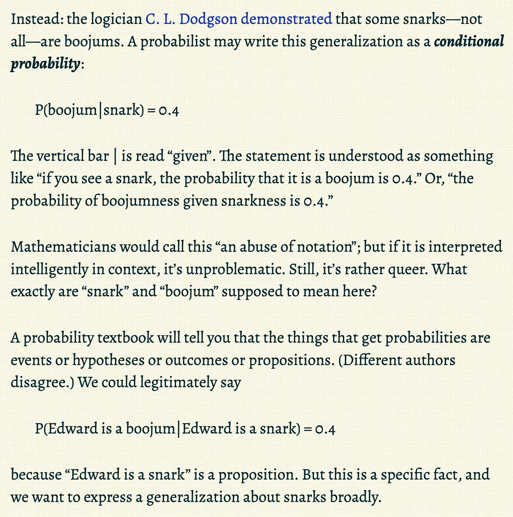
This is a warmup. We have
$$
P(\bo\mid\sn)
$$
which is just straight forward probability, except that Chapman does not define any random variables. Let’s go ahead and do that for him. Chapman notes that it would not be agreed upon exactly how to formalize $P(\bo \mid \sn)$, but I think that there is a fairly canonical interpretation.
Clearly we have a 2x2 probability table, where the columns are $\bo$ is true vs false, and the rows are $\sn$ is true vs false. For example (and I’m just filling in arbitrary probabilities):
| $\bo$ | $\neg\bo$ | |
|---|---|---|
| $\sn$ | 0.4 | 0.05 |
| $\neg\sn$ | 0.1 | 0.45 |
Perhaps this is a sub-table, i.e. part of a larger table containing information we are marginalizing over. But no matter what, we have a sample set $\O$, and some process has selected the latent outcome $\o\in\O$. Then $\o$ encodes within it all the information me might want to know, i.e. whether $\bo$ and $\sn$ are respectively true.
Perhaps we are selecting one instance of a thing which may or may not be a snark and may or may not be a boojum. If we assert $P(\bo \mid \sn) = 0.4$, what we are actually saying is that if a snark is drawn, then its probability of being a boojum is always 0.4.
It will help to actually formalize Chapman’s examples. I will use random variables. Here, $\r{\bo},\r{\sn} : \O \to \bool$ become random variables that take in $\o$, which contains information about the thing that the random process drew, and tell us the properties we care about.
$$
\begin{aligned}
P(\r{\bo} \mid \r{\sn}) &= \frac{P(\set{\o\in\O \mid \r{\bo}(\o)} \cap \set{\o\in\O \mid \r{\sn}(\o)})}{P\set{\o\in\O \mid \r{\sn}(\o)}} \\
& = \frac{P\set{\o\in\O \mid \r{\bo}(\o) \and \r{\sn}(\o)}}{P(\r{\sn}^{-1}(\1))} \\
& = P((\r{\bo} \and \r{\sn}^{-1})(\1))/\mc{Z}\,.
\end{aligned}
$$
We are merely adding up all the probability that $\o$ is a snark and boojum (the probability of drawing a thing that is a snark and boojum), and then rescaling by the probability that $\o$ is a snark so that the probability across snark things sums to 1. The important point is that we are marginalizing away all other information contained in $\o$. It is certainly possible that some kinds of snarks are likely to be boojums, while other kinds are not. Then we are averaging over those two cases. If you conditioned on extra information that distinguishes these two types of snarks, the probability of being a boojum would go up or down.
So under this interpretation, all properties/predicates are referring to a single instance of a thing drawn randomly by some process. I feel that is the simplest interpretation, though it is certainly not the only. But let’s run with it.
Next, Chapman wants us to make sense of the statement
$$
\fa x: P(\bo(x)|\sn(x)) = 0.4
$$
We are re-introduced to $\bo$ and $\sn$ as predicates (i.e. Boolean-valued functions) on the domain $\mon$ (apparently boojums and snarks are monsters). Unlike before, we can have two different instances of things that exist simultaneously, $x,y\in\mon$, and then ask about $\bo(x),\bo(y),\sn(x),\sn(y)$. This changes our interpretation. Before, I assumed we selected one thing out a space of possibilities. Now, we have an entire set of things, $\mon$ (possibly an infinity of them), that we can arbitrarily query simultaneously, e.g. $\bo(x) \and \neg \bo(y) \or (\neg \sn(x) \and \sn(y)) \or \bo(z)$ for some $x,y,z\in\mon$. We can talk about all things all at once using quantifiers:
$$
\fa x \in \mon : \sn(x) \implies \bo(x)\,,
$$
or perhaps
$$
\ex x \in \mon : \sn(x) \and \neg \bo(x)\,.
$$
So what is being randomly drawn here? Clearly not the things (monsters), because they all exist at once. Let’s consider the truth table,
| Monster | snark | boojum |
|---|---|---|
| Edward | True | True |
| Zachary | True | False |
| $\vdots$ | $\vdots$ | $\vdots$ |
| $x_i$ | False | True |
| $\vdots$ | $\vdots$ | $\vdots$ |
This lists out the truth values of the same predicates on every thing in $\mon$. Now imagine that we randomly select one of these (possibly infinitely long) tables, meaning that there is a joint probability distribution over every truth value in the table.
Now we can make sense of Chapman’s example. Let’s rewrite it with random variables:
$$
\fa x \in \mon: \tup{P(\r{\bo}(x)|\r{\sn}(x)) = 0.4}
$$
I’m making the predicates random variables, $\r{\bo},\r{\sn} : \O \to (\mon \to \bool)$, i.e. function-valued functions (see my discussion towards the top of this article if that confuses you). $\r{\bo}$ and $\r{\sn}$ take in a randomly chosen state $\o$ which contains all the truth values in our truth table above ($\O$ contains all possible such tables), and these random variables output a function which takes in a thing and returns a Boolean. Another way to think about it is that $\r{\bo}(\o)$ is a function that lets you retrieve a value from a specific row in the truth table, where the row is identified by a $\mon$ instance which you pass as input. In a sense, $\r{\bo}(\o)$ is a database query function, and $\o$ is the database (think MySQL table).
The statement above unpacks into
$$
\begin{aligned}
& \fa x \in \mon: \tup{P(\r{\bo}(x)|\r{\sn}(x))=0.4} \\
&\quad= \fa x \in \mon: \tup{P(\set{\o\in\O \mid \r{\bo}(\o)(x)} \cap \set{\o\in\O \mid \r{\sn}(\o)(x)})/\mc{Z} = 0.4} \\
&\quad= \fa x \in \mon: \tup{P\set{\o\in\O \mid \r{\bo}(\o)(x) \and \r{\sn}(\o)(x)}/\mc{Z} = 0.4}\\
&\quad= \fa x \in \mon: \tup{P((\r{\bo}(x) \and \r{\sn}(x))^{-1}(\1))/\mc{Z} = 0.4}\,,
\end{aligned}
$$
where $\mc{Z} = P\set{\o\in\O \mid \r{\sn}(\o)(x)}$.
This might be a headache to wrap your head around, but it’s mathematically well formed. This is simply saying that, for every monster, if we randomly pick a truth table on which it’s a snark, the propability that it’s also a boojum on that table is 0.4 [edit: thank you bunthut for correcting my description here]. Again we are marginalizing over additional information that might be in the table (e.g. other columns), so this is true on average.
Inferring a generality from instances
Chapman wants to know how Bayesian probability let’s you infer generalities from specific instances. Suppose we observe
$$
\r{\obs} = \r{\sn}(\ed) \and \r{\bo}(\ed)\,.
$$
Here $\r{\obs}$ is a random variable because it is composed of random variables (we could say it’s a proposition-valued random variable), i.e. it is the function $\r{\obs}(\o) = \r{\sn}(\o)(\ed) \and \r{\bo}(\o)(\ed)$. To condition on the set $\r{\obs}^{-1}(\1) = \set{\o\in\O \mid \r{\obs}(\o)}$ means to perform a domain restriction to all $\o$ encoding probability tables with that have the row:
| Monster | snark | boojum |
|---|---|---|
| Edward | True | True |
Now we may ask, does the probability that all snarks are boojums go up if we condition on our observation that Edward is a snark and a boojum? Formally,
$$
\begin{aligned}
&P(\fa x \in \mon : \r{\sn}(x) \implies \r{\bo}(x) \mid \r{\obs}) \\
&\quad \overset{?}> P(\fa x \in \mon : \r{\sn}(x) \implies \r{\bo}(x))\,.
\end{aligned}
$$
The short answer is that this depends on $P$. To see exactly how $P$ determines our ability to update our beliefs about generalities, it is instructive to take a detour to talk about coin tossing.
Interlude: A tale of infinite coin tosses
A probability distribution on truth tables can be equivalently viewed as a random process that draws a sequence of binary outcomes. It is customary to call such a process a sequence of coin tosses, though these abstract “coins” are not necessarily independent, and can have arbitrary dependencies between their outcomes.
I want to point out that for finite truth tables, which I will call a finite domain, 0th order logic and 1st order logic have equivalent power, because quantifiers can be rewritten as finite conjunctions or disjunctions in the 0th order language, i.e. $\fa x : f(x) = f(x_1) \and \ldots \and f(x_n)$. Chapman agrees that Bayesian inference could be said to “extend” 0th order logic, so this works as expected. Our interest is really in infinite domains, i.e. infinitely long truth tables, i.e. infinitely many monsters. I’m going to assume countable infinity which demonstrates a non-trivial difference between 0th order and 1st order Bayesian inference (beyond countable infinity things get even weirder and harder to work with). Note that in a countably infinite domain we are already working with uncountable $\O$ (e.g. the set of all infinitely long truth tables or infinite coin tosses).
In finite domains, observing an instance of $f(x_1)$ being true, for some $x_1$, makes you more confident of $\fa x : f(x)$, unless you put 0 marginal prior probability on $f(x_1)$ or 0 prior probability on $\fa x : f(x)$. This is Bayesian 0th order logic.
In a countably infinite domain, observing an instance of $f(x_1)$ (or finitely many of them) may or may not change your confidence of $\fa x : f(x)$. It really depends on your prior.
This is analogous to predicting whether an infinite sequence of coin tosses (again I really just mean some random process with binary outputs) will all come up heads based on the observation that the $n$ tosses you observed all came up heads. Remember that the tosses may be causally dependent. Let our sample set be $\O = \B^\infty = \set{0,1}^\infty$, the set of all countably infinite binary sequences (where 1 is a head and 0 is a tail). For $\o \in \O$, let $\o_{1:n}$ denote the finite length-$n$ prefix of $\o$. Given we observe $\o_{1:n}$, what is the probability that $\o = 111111\ldots$ (an infinite sequence of 1s)? Let’s write this formally using random variables:
$$
P(\r{X}_{n+1:\infty} = 111111\ldots \mid \r{X}_{1:n} = 111111\ldots)\,,
$$
where $\r{X}\_i : \O \to \B : \o \mapsto \o_i$ is the random variable for the $i$-th toss, and $\r{X}\_{i:j} = (\r{X}\_i, \r{X}\_{i+1}, \ldots, \r{X}\_{j-1}, \r{X}\_j)$ is the random variable for the sequence of tosses from $i$ to $j$ (inclusive).
Suppose for all $i \in \N$, $P(\r{X}\_i = 1) = \th$. Let’s call this a Bernoulli prior. (By the way, a perfectly natural use of a quantifier with probability.) Then the tosses are independent, and $P(\r{X}\_{1:n} = 111111\ldots) = \th^n$. Furthermore,
$$
P(X_{1:\infty}=111111\ldots) = \lim_{n\to\infty} P(\r{X}_{1:n} = 111111\ldots) = \lim_{n\to\infty}\th^n\,,
$$
which equals $0$ iff $0 \leq \th < 1$ and equals $1$ iff $\th = 1$. If we model the tosses as being i.i.d., unless we are certain that all tosses will be heads, we place 0 prior probability on that possibility, even if the probability that any toss will be heads is very close to 1. Of course, the probability of any infinite sequence occurring will also be 0. This would imply that we really cannot say anything about an infinity of outcomes using this prior.
However, we are free to choose some other kind of prior. In fact, an i.i.d. prior, such as the Bernoulli prior, does not update beliefs even on finite outcomes, because
$$
P(\r{X}_j = 1 \mid \r{X}_i = b_i) = P(\r{X}_j = 1) = \theta\,.
$$
This means, a prior where learning-from-data can take place is necessarily non-i.i.d. w.r.t. the “coin tosses”. That is to say, if we want to be able to learn, we want to choose a $P$ where for most $i$ and $j$,
$$
P(\r{X}_j = 1 \mid \r{X}_i = b_i) \neq P(\r{X}_j = 1)\,.
$$
As a side note, this does not mean the random process in question cannot be i.i.d. Bernoulli. If we consider the uniform mixture of Bernoulli hypotheses,
$$
P(\r{X}_{1:n} = b_{1:n}, \r{\Theta}=\theta) = \theta^{\sum_i b_i}(1-\theta)^{n-\sum_i b_i}\,,
$$
then $P(\r{X}\_{1:n} = b\_{1:n})$ is the marginal Bayesian data distribution, which is certainly not i.i.d. w.r.t. $\r{X}\_1, \ldots, \r{X}\_n$ (checking this is left as an exercise to the reader). That is what allows you to grow more confident about the behavior of future outcomes (and thus grow more confident about $\theta$) as you observe more outcomes.
Question: What kind of prior would make us more confident that all tosses will be heads from a finite observation? The answer is simple: a prior that puts non-zero probability $\phi$ on infinite heads, i.e.
$$
P(X_{1:n}=111111\ldots) \xrightarrow{n\to\infty} \phi
$$
for $0 < \phi < 1$. That also means the probability of getting any other infinite sequence that is not all heads is exactly $1-\phi$. It also means the first few observations of heads are the most informative, and then we get diminishing returns, i.e.
$$
P(\r{X}_{n+1:\infty} = 1_{1:\infty} \mid \r{X}_{1:n} = 1_{1:n}) = \frac{P(\r{X}_{1:\infty} = 1_{1:\infty})}{P(\r{X}_{1:n} = 1_{1:n})} = \frac{\phi}{P(\r{X}_{1:n} = 1_{1:n})}\,.
$$
(switching to the shorthand $1\_{1:\infty} = 111111\ldots$) Since $P(\r{X}\_{1:n} = 1\_{1:n})$ converges to $\phi$, then $\phi/P(\r{X}\_{1:n} = 1\_{1:n})$ must converge to 1, and so the probability that the remaining infinite sequence of tosses will all be heads given the first $n$ tosses were heads converges (upwards) to 1 as $n\to\infty$. This makes sense, since if you can infer an infinite sequence from finite data, then the infinite sequence contains finite information. Stated another way, the surprisal (i.e. information gain) $-\lg P(\r{X}\_{1:\infty} = 1\_{1:\infty}) = \lg\frac{1}{\phi}$ for observing the infinite sequence $1\_{1:\infty}$ is finite, and that finite information gain is spread asymptotically across the infinite sequence, i.e. your future information gain diminishes to 0 as you observe more 1s.
Such a prior essentially says that knowledge of infinite heads is finite information to me (or whatever agent uses this prior). That can only be true if I have the privileged knowledge that infinite heads is a likely possibility. If I expect infinite heads (with any probability), then observing finite heads confirms that expectation.
Another way to think about it is, I can only put non-zero probability on countably many infinite sequences out of an uncountable infinity of them (there is one infinite binary sequence for every real between 0 and 1). Any infinite sequence (e.g. all heads) with non-zero probability is being given special treatment.
I think what Chapman is trying to get at is that Bayesian inference is doing something trivial. You can’t get something from nothing. Your prior is doing all the epistemological heavy lifting. Within the confines of a model, you can know that something is true for all $x$, but in the real world you cannot reasonably know something is true in call cases (unless you can prove it logically, but then it would be a consequence of your chosen axioms and definitions). In that case, we might say that a prior that asserts that there is some non-zero probability of getting infinite heads is an unreasonable one, or at least very biased. Removing such priors then means we cannot infer an infinite generality from specific instances.
To reiterate, Bayesian inference just tells you what you already claim to know: “hey your prior says you can infer a generality from specific instances, so I’ll update your beliefs accordingly” vs “your prior models infinitely many instances of $f(x)$ as being independent, so I cannot update your belief about the generality from finitely many instances”. People who view Bayesian inference as the end-all be-all to epistemology are hiding the big open problems in their choice of prior. Chapman appears to be suggesting (and I agree) that the hard problems of epistemology have never really been solved, and we should acknowledge that.
Getting back to boojums and snarks, it should be straightforward to see how $P(\fa x \in \mon : \r{\sn}(x) \implies \r{\bo}(x) \mid \r{\obs})$ would work. Supposing $\mon$ is an infinite set, then if our prior put some non-zero probability on the infinite tables where $\fa x \in \mon : \sn(x) \implies \bo(x)$ is true, then observing that finitely many observations conform to this hypothesis should make our conditional probability go up. On the other hand, if we don’t use such an epistemically strong prior, then the probability of observing an infinite table filled with “True” is 0 - the same probability of observing any individual infinite table. Zero-probability outcomes can never become non-zero just by conditioning on something.
Probability inside a quantifier inside a probability
Chapman writes,
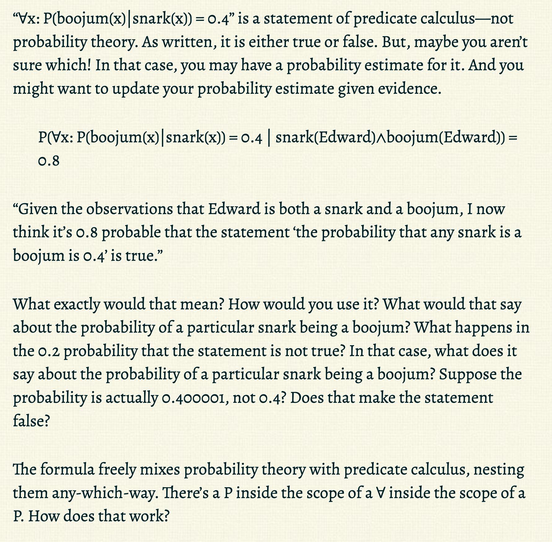
Why are we not sure about whether “∀x: P(boojum(x)|snark(x)) = 0.4” is true? If we’ve fully defined $\O$ and $P$ and our random variables, $\r{\bo}$ and $\r{\sn}$, then we should be able to determine whether this is true, barring undecidability or computational intractibility, which I’ll classify as logical uncertainty.
I think Chapman is asking: how can observing that Edward is a snark and a boojum should increase our probability that any snark is also a boojum? I agree that the example Chapman gives wouldn’t accomplish this, but let me construct a similar expression that would:
$$
\begin{aligned}
&\fa x \in\mon\setminus\set{\ed} : \\
&\qquad P(\r{\bo}(x) \mid \r{\sn}(x) \and \r{\sn}(\ed) \and \r{\bo}(\ed)) \\
&\qquad \overset{?}> P(\r{\bo}(x) \mid \r{\sn}(x))\,.
\end{aligned}
$$
Whether this is true will depend on what kind of prior $P$ we choose (see the coin tossing discussion above).
Chapman also claims that nesting a probability inside a quantifier inside a probability, as he does in his example, cannot work. I agree with Chapman that nesting $P$ inside $P$ generally doesn’t make sense, though technically his example will parse to something if we make the usual random variable replacements I’ve been making above.
However, nesting different measures can make sense. Suppose we didn’t want to settle for one $P$, and instead we had a set $\mc{M}$ of measures $\mu$ on $\O$. In the Bernoulli coin toss example above, $\mc{M}$ is the set of all i.i.d. Bernoulli measures infinite coin tosses. To make a prediction, we average the predictions across $\mu\in\mc{M}$ according to our hypothesis prior, which is a measure $\pi$ on $\mc{M}$. Let’s define $P$ as the derived measure on $\mc{M}\times\O$, i.e.
$$
P(\r{\mu} = \mu, \r{\o} = \o) = \pi\set{\mu}\cdot \mu\set{\o}\,.
$$
(Technically this expression would often be 0 since $\O$ is uncountable, but hopefully you get the idea.)
The expression of interest becomes
$$
P\tup{\fa x \in\mon : \r{\mu}(\r{\bo}(x) \mid \r{\sn}(x)) = 0.4 \Mid \r{\sn}(\ed) \and \r{\bo}(\ed)}
$$
where $\r{\mu}: \mc{M}\times\O \to \mc{M} : (\mu,\_) \mapsto \mu$ is a measure-valued random variable, and $\r{\bo},\r{\sn} : \O \to (\mon \to \bool)$ are the usual predicate-valued random variables on $\O$, that means they are random variables for the inner measure $\r{\mu}$.
In words, this expression is asking for the $P$-probability of all $(\mu,\o) \in \mc{M}\times\O$ s.t. $\fa x \in\mon : \mu(\r{\bo}(x) \mid \r{\sn}(x)) = 0.4$ holds, restricted to truth tables $\o$ where $\r{\sn}(\o)(\ed) \and \r{\bo}(\o)(\ed)$ is true.
This is actually a reasonable query to make. Going back to the Bernoulli coin tossing example, if we observe the first coin toss is heads ($b_1 = 1$), that will put more posterior probability on hypotheses $\theta$ where 1 is more likely than 0, i.e.
$$
P(\r{\Theta} > 0.5 \mid \r{X}_1 = 1) > P(\r{\Theta} > 0.5)\,.
$$
In general we can ask some arbitrary question about the posterior probability (after making in observation) of some hypotheses satisfying a query, i.e.
$$
P(\mathrm{predicate}(\r{\Theta}) \mid \r{X}_1 = 1)\,,
$$
where $\mathrm{predicate} : \Theta \to \bool$ is some Boolean-valued function of Bernoulli parameter $\theta$. That predicate can involve a quantifier and the data probability under hypothesis $\theta$. For example, we can reenact the same example above:
$$
P(\fa i \in \set{2,3,\ldots} : P(\r{X}_i = 1 \mid \r{\Theta}) > 0.5 \mid \r{X}_1 = 1)\,.
$$
This is the $P$-probability of all $(\theta, b_{1:\infty}) \in \Theta\times\B^\infty$ s.t. the probability of every future outcome under the $\theta$-hypothesis is greater than 0.5, restricted to coin toss sequences $b_{1:\infty}$ where $b_1 = 1$. I do expect this probability to be larger than $P(\fa i \in \set{2,3,\ldots} : P(\r{X}_i = 1 \mid \r{\Theta}) > 0.5)$ (not conditioning on data) if I expect that hypotheses where the probability of heads is greater than a half (i.e. $P(\r{X}_i = 1 \mid \r{\Theta}=\theta) > 0.5$) will get upweighted by observing a head.
Probability precision (part II)
Quick side note regarding the question
Suppose the probability is actually 0.400001, not 0.4? Does that make the statement false?
Yes. This “paradox” of probability on continuous sets is straight out of probability 101. The probability of drawing a real number uniformly from the unit interval is 0. What you actually care about is the probability of drawing a real number in some subinterval. In this case,
$$
P(\r{\bo}(x) \mid \r{\sn}(x)) \in (0.4-\vep, 0.4+\vep)
$$
is acceptable, and we can choose whatever precision $\vep$ we want.
Final boss
$$
\newcommand{\eql}{\mathrm{equal}}
\newcommand{\lts}{\mathrm{looksTheSame}}
\newcommand{\dna}{\mathrm{DNA\_match}}
\newcommand{\obs}{\mathrm{observations}}
\newcommand{\ar}{\mathrm{Arthur}}
\newcommand{\ha}{\mathrm{Harold}}
$$
I believe at this point I’ve covered everything Chapman points out as being ill-posed, namely, arbitrary nesting of probability expressions and quantifiers, and “learning” about generalities from specific instances.
Chapman gives a more involved example that I think is more of the same idea, but I will go through it just for fun. Chapman writes,
Let’s run with same interpretation as before - we are randomly drawing a truth table where the rows are instances of $\mon$ and the columns are predicates.
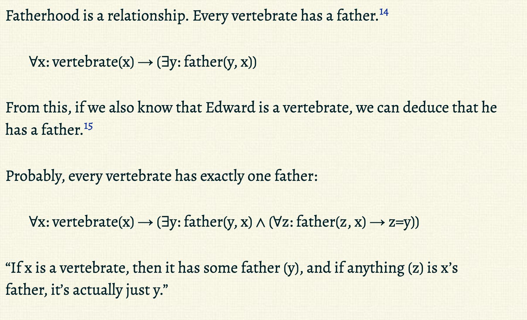
It is not clear whether Chapman is asserting, or querying, that the following is true:
$$
\fa x : \ve(x)\implies (\ex y : \fr(y,x) \and (\fa z : \fr(z,x) \implies z=y))\,,
$$
i.e. is Chapman telling us that this is true, or is he querying whether it is true. If we take the predicates here to be columns in a truth table, then this proposition’s truth value depends on the entries of the truth table. Technically we need two tables, one for single-argument properties and one for two-argument properties:
| Monsters | vertebrate |
|---|---|
| $x_1$ | True |
| $x_2$ | False |
| $\vdots$ | $\vdots$ |
and
| Argument-1 | Argument-2 | father |
|---|---|---|
| $x_1$ | $y_1$ | True |
| $x_1$ | $y_2$ | False |
| $x_2$ | $y_1$ | False |
| $x_2$ | $y_2$ | True |
| $\vdots$ | $\vdots$ | $\vdots$ |
Rewriting with random variables, we have:
$$
\begin{aligned}
& \fa x \in \mon : \\
&\qquad \r{\ve}(x)\implies \\
&\qquad\qquad \ex y \in \mon: \r{\fr}(y,x) \and (\fa z \in \mon: \r{\fr}(z,x) \implies z=y)\,.
\end{aligned}
$$
Again, our random variables are function-valued, $\r{\ve} : \O \to (\mon \to \bool)$ and $\r{\fr} : \O \to (\mon^2 \to \bool)$. Each $\o\in\O$ contains the two tables above (and maybe other information), and $\O$ contains all such combination of tables.
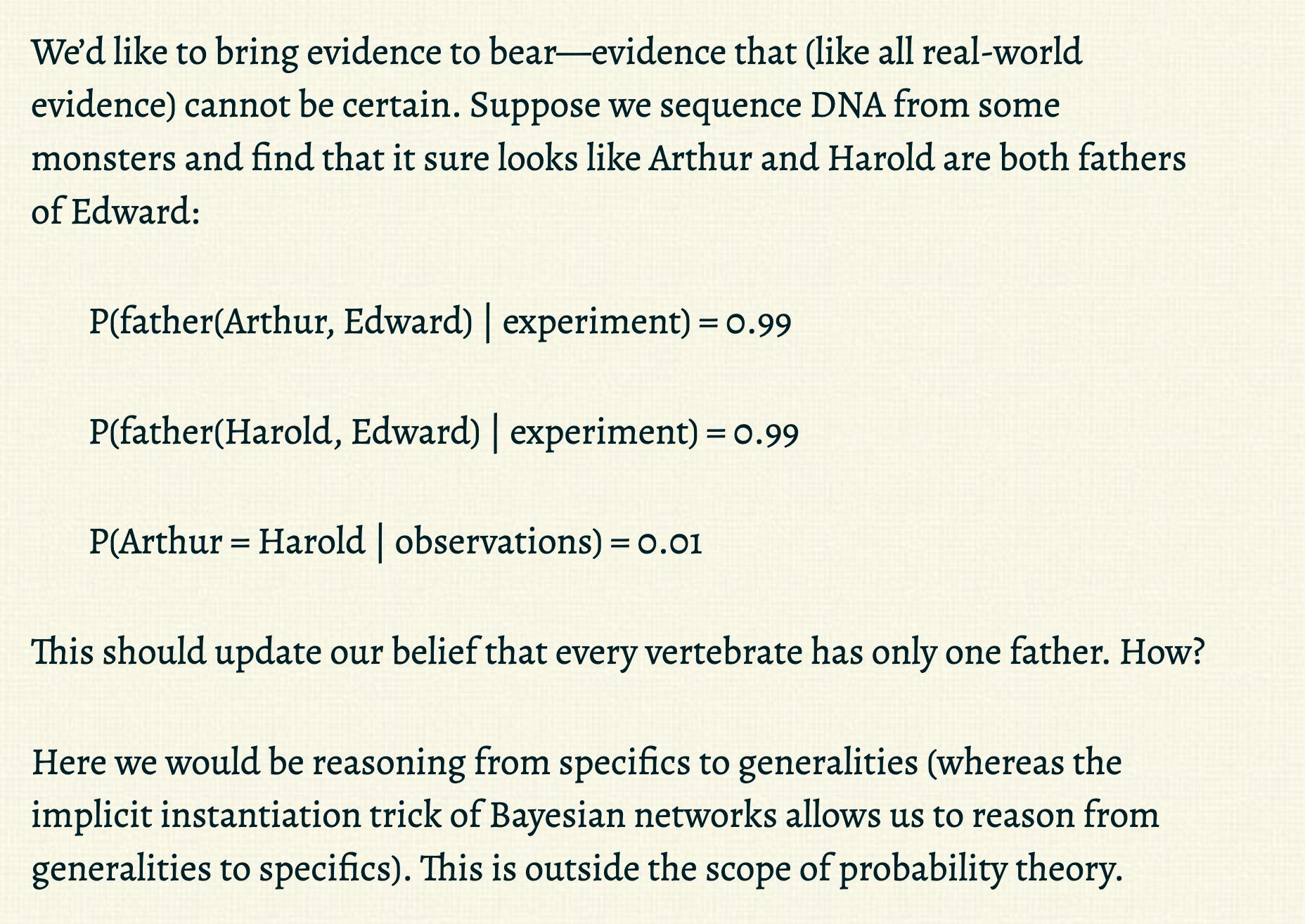
Now Chapman asks how observing specific data can update the truth values of specific propositions. He supposes that “we sequence DNA from some monsters and find that it sure looks like Arthur and Harold are both fathers of Edward.”
Chapman wants to evaluate the following:
But Chapman doesn’t provide the formal definition of experiment or observation. From context clues, I will infer reasonable definitions.
First, we need a way to talk about DNA matches. I’ll invoke a random variable $\r{\dna} : \O \to (\mon^2 \to \bool)$ which is the outcome of a DNA experiment (match or no match) run on $x$ and $y$.
Next, the last expression $P(\ar = \ha \mid \obs)$ implies that one monster can go by two different names. If we regard the set $\mon$ to be a set of names, not the identities of monsters, then we can have uncertainty about the equality of two different names. I’ll invoke the random variable $\r{\eql} : \O \to (\mon^2 \to \bool)$ that returns true if the given names are actually the same monster.
Now the two-argument truth table contains the corresponding extra columns (remember that $\o$ contains an entire such truth table and the one-argument table above):
| Argument-1 | Argument-2 | father | equal | DNA_match |
|---|---|---|---|---|
| $x_1$ | $y_1$ | True | True | False |
| $x_1$ | $y_2$ | False | False | False |
| $x_2$ | $y_1$ | False | False | False |
| $x_2$ | $y_2$ | True | True | True |
| $\vdots$ | $\vdots$ | $\vdots$ | $\vdots$ |
We can write our data as follows:
$$
\r{\obs} = \r{\dna}(\ar, \ed) \and \r{\dna}(\ha, \ed)\,.
$$
Note that $\r{\obs} : \O \to \bool$ is itself a random variable, being composed of random variables.
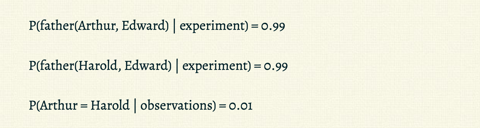
Then we can rewrite Chapman’s expressions:
$$
\begin{aligned}
&P(\r{\fr}(\ar, \ed) \mid \r{\dna}(\ar, \ed)) &= 0.99 \\
&P(\r{\fr}(\ha, \ed) \mid \r{\dna}(\ha, \ed)) &= 0.99 \\
&P(\r{\eql}(\ar, \ha) \mid \r{\obs}) &= 0.01
\end{aligned}
$$
I replaced $\ar = \ha$ with $\r{\eql}(\ar, \ha)$, our monster equality random variable (to distinguish from name equality).
From top to bottom, $P(\r{\fr}(\ar, \ed) \mid \r{\dna}(\ar, \ed)) = 0.99$ says that in 99% of truth tables (as measured by $P$; my language here doesn’t imply $P$ has to be uniform, but the idea of a measure is that it tells you how much of something you have) where $\ar$ and $\ed$ DNA match, $\ar$ is $\ed$’s father. Likewise for the middle expression. The last expression, $P(\r{\eql}(\ar, \ha) \mid \r{\obs}) = 0.01$, says that for only 1% of truth tables (as measured by $P$) where $\ar$ and $\ha$ both DNA match $\ed$ and $\ha$, it is the case that $\ed$ and $\ha$ are actually distinct monsters ($\ed$ has two fathers). Why is that? Would the DNA tests be likely to be wrong in that scenario?
I think Chapman actually wanted to say that the probability of our observations is low,
$$
P(\r{\obs}) = 0.01\,,
$$
but given this observation the probability that Edward has two fathers is high, which can allows us to update our belief about vertebrates having two fathers.
Chapman wants to know, is the following meaningful?
$$
\begin{aligned}
& P(\fa x \in \mon : \\
&\qquad \r{\ve}(x)\implies \\
&\qquad\qquad \ex y \in \mon: \r{\fr}(y,x) \and (\fa z \in \mon: \r{\fr}(z,x) \implies \r{\eql}(z, y)) \\
&\quad\mid \r{\obs})
\end{aligned}
$$
Does conditioning on $\r{\obs}$ change the probability that all vertebrates have one father? Are we magically somehow inferring a generality from specific instances, just by virtue of the machinery of probability theory and set theory? While this monstrosity of an equation (pun intended) may be syntactically correct, how do we interpret what it’s doing?
This example is fundamentally the same as the infinite coin tossing example. If we choose a prior that puts non-zero probability on monsters having two fathers, then I expect that updating on observations which are supported by that hypothesis causes the 2-father hypothesis to become more likely. If you choose a prior where no monster can have two fathers, then you cannot update yourself out of that assumption.
Something I think Chapman is trying to get at, is that you cannot update your beliefs on data within the Bayesian framework without first specifying how your beliefs interact with data. Given any Bayesian probability distribution, you cannot pop out a level of abstraction and start updating that Bayesian model itself on data, unless you had the foresight to nest your Bayesian model inside an even larger meta-model that you also defined up front. I’m merely demonstrating that you can define the meta-model if you want to. I do acknowledge that we have a problem of infinite regress, and you need to keep creating ever more elaborate meta-models whenever you want to explain how an rational person should update their ontology given their experience (or you can use Solomonoff induction, i.e. Bayesian inference on all (semi)computable hypotheses).