[This is a note, which is the seed of an idea and something I’ve written quickly, as opposed to articles that I’ve optimized for readability and transmission of ideas.]

$$
\newcommand{\mb}{\mathbb}
\newcommand{\mc}{\mathcal}
\newcommand{\E}{\mb{E}}
\newcommand{\B}{\mb{B}}
\newcommand{\kl}[2]{D_{KL}\left(#1\ \| \ #2\right)}
\newcommand{\argmin}[1]{\underset{#1}{\mathrm{argmin}}\ }
\newcommand{\argmax}[1]{\underset{#1}{\mathrm{argmax}}\ }
\newcommand{\abs}[1]{\left\lvert#1\right\rvert}
\newcommand{\atup}[1]{\left\langle#1\right\rangle}
\newcommand{\set}[1]{\left\{#1\right\}}
\newcommand{\t}{\theta}
\newcommand{\T}{\Theta}
\newcommand{\p}{\phi}
\newcommand{\r}{\rho}
$$

Previous attempts:

In Free Energy Principle 1st Pass, I used a tutorial to try to understand the free energy formalism. I figured out the “timeless” and actionless case, but I became confused when actions and time were added.
In , I tried to translate between the formalism presented in https://danijar.com/apd/ (which is a deep learning collaboration between Danijar Hafner and Karl Friston) and the tutorial tutorial. I also tried to make the connection to Solomonoff induction.
In Variational Solomonoff Induction, I thought about whether free energy (as variational inference) could be applied to deep program synthesis to approximate Solomonoff induction.

Using the same tutorial as before, A Step-by-Step Tutorial on Active Inference and its Application to Empirical Data, I will go through the free energy formalism again and try to work out time and actions.

Review

To recap what I figured out in Free Energy Principle 1st Pass:

Suppose $o\in\mc{O}$ is the observation space and $s\in\mc{S}$ is the hypothesis/state space (to use the notation of the tutorial). For now, let’s assume that $\mc{S}$ is the hidden state space of the environment in some timestep. $p(o,s)$ is the agent’s model of the environment, relating observations to hidden states, and the prior probability of the environment being in any particular hidden state. Let’s also ignore questions about the meaning of these probabilities (objective or subjective) and where they come from. If it’s easier to think about, assume these probabilities are subjective.

If $o$ is observed (one timestep only), then we want to calculate the posterior probability $p(s\mid o)$ of each $s\in\mc{S}$. If this is intractable to do, we can instead find an approximation $q_o(s)$:

$$
q_o := \argmin{q \in \mc{Q}} \kl{q(s)}{p(s\mid o)}
$$

where $\mc{Q}$ is some space of distributions that you choose $q_o$ from. Presumably $\mc{Q}$ is restricted somehow, otherwise the solution is $q=p$ in which case you are doing exact Bayesian inference.

$$
\begin{aligned}
\kl{q(s)}{p(s\mid o)} &= \E_{s\sim q}\left[\lg\frac{q(s)}{p(s\mid o)}\right] \\
&= \E_{s\sim q}\left[\lg\frac{q(s)}{p(s)}\right] + \E_{s\sim q}\left[\lg \frac{1}{p(o \mid s)}\right] + \E_{s\sim q}[p(o)]\\
&= \kl{q(s)}{p(s)} - \E_{s\sim q}\left[\lg p(o \mid s)\right] - \lg\frac{1}{p(o)} \\
&= \mc{F}[q] - \lg\frac{1}{p(o)}\,,
\end{aligned}
$$

where

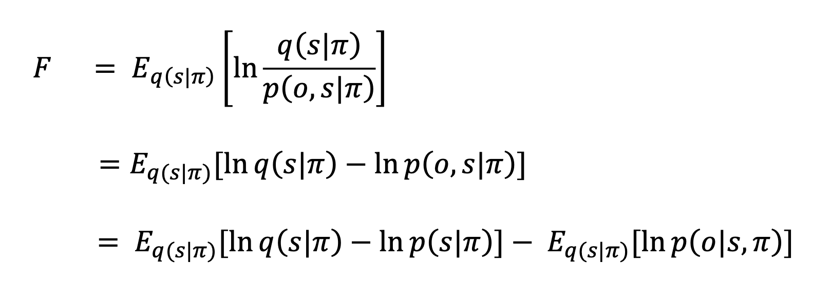
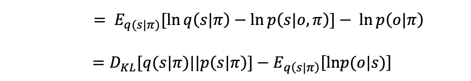
$$
\begin{aligned}
\mc{F}[q] &= \kl{q(s)}{p(s)} - \E_{s\sim q}[\lg p(o \mid s)]\\
&= \E_{s\sim q}\left[\lg\frac{q(s)}{p(s,o)}\right]
\end{aligned}
$$

is called variational free energy. $\kl{q(s)}{p(s)}$ is called accuracy and $\E_{s\sim q}[\lg p(o \mid s)]$ is called complexity. $\lg\frac{1}{p(o)}$ is called surprise (self-information of the observation $o$).

Minimizing $\mc{F}[q]$ w.r.t. $q$ minimizes $\kl{q(s)}{p(s\mid o)}$. The surprise $\lg\frac{1}{p(o)}$ is constant w.r.t. this minimization. (Remember this is all assuming $o$ is given and fixed.)

New stuff

In the tutorial, we have free energy defined just as in my notes, except that everything now depends on policy $\pi$:

The policy $\pi$ is a probability distribution over actions (, e.g. $\pi(a_t \mid o_{1:t}, a_{1:t-1})$. More on that later.

Interaction loop

It is not clear to me whether $o,s$ are sequences over time, or just one time-step. In Variational Solomonoff Induction I showed how to interpret $s$ as a hypothesis that explains an infinite sequence of observations, i.e. $s$ is not a sequence but $o$ is. When I write $o_{1:\infty}$, that is an observation sequence over time. When I write $s_{1:\infty}$ that is a state sequence over time. I’ll use $h$ later to denote a time-less hypothesis on observation sequences $o_{1:\infty}$.

Let’s unpack the agent-environment interaction loop. Given policy $\pi$,

$$
p(o_{1:\infty},s_{1:\infty}\mid\pi) = \sum_{a_{1:\infty}}\prod_t p(o_t,s_t\mid a_t,s_{t-1})\pi(a_t\mid o_{1:t-1},a_{1:t-1})
$$

where $p(o_t,s_t\mid a_t,s_{t-1})$ is the probability of next observation and hidden state given input action $a_t$ and previous state, and $\pi(a_t\mid o_{1:t-1},a_{1:t-1})$ is the probability of the agent taking action $a_t$ given its entire history $o_{1:t-1},a_{1:t-1}$ (alternative we can give the agent internal state and condition on that).

On the other hand, if $s$ (or $h$) is a time-less hypothesis: then we have

$$
p(o_{1:\infty},h\mid\pi) = \sum_{a_{1:\infty}}\prod_t p(o_t\mid a_{1:t},o_{1:t-1},h)p(h)\pi(a_t\mid o_{1:t-1},a_{1:t-1})
$$

where $p(h)$ is the prior on hypothesis $h$.

Below, I will leave it ambiguous whether $s$ is a sequence of states or a time-less hypothesis. The math should be the same either way.

Active inference

How are actions chosen? This is the big question I could not penetrate in my previous attempts. From the tutorial:

When inferring optimal actions, however, one cannot simply consider current observations. This is because actions are chosen to bring about preferred future observations. This means that, to infer optimal actions, a model must predict sequences of future states and observations for each possible policy, and then calculate the expected free energy (𝐸𝐹𝐸) of those different sequences of future states and observations.

This is talking about taking an expectation over future states and observations. Let’s assume $p(o_{1:\infty}, s_{1:\infty} \mid \pi)$ is the true environment dynamics. We are introduced to a new term $q(o_{1:\infty}\mid\pi)$ which are the agent’s observation preferences over time given a particular policy.

The text is saying we want to choose policy $\pi$ to maximize $G(\pi)$. What’s troubling is that there is another term, $p(\pi)$, a prior over policies. If we are choosing policies freely, what does this prior represent?

The text says that the preferred policy also minimizes free energy:

Since ‘preferred’ here formally translates to ‘expected by the model’, then the policy expected to produce preferred observations will be the one that maximizes the accuracy of the model (and hence minimizes 𝐸𝐹𝐸).

Exact inference

To simplify things, let’s suppose the agent can do perfect Bayesian inference, so that $q_o(s\mid\pi) = p(s \mid o,\pi)$. Let’s see what happens if we plug in $p(s\mid o,\pi)$ for $q_o(s\mid \pi)$ in our free energy definition:

$$
\mc{F} = \E_{s \sim p(s\mid o,\pi)}\left[\lg \frac{p(s\mid o,\pi)}{p(s,o\mid\pi)}\right] = \E_{s \sim p(s\mid o,\pi)}\left[\lg \frac{1}{p(o\mid \pi)}\right] = \lg \frac{1}{p(o\mid \pi)}
$$

which is just the surprise (i.e. self-information due to observing $o$). Minimizing free energy means choosing $\pi$ to maximize the data likelihood:

$$
\pi^* := \argmax{\pi} p(o\mid\pi)
$$

Remember that $\mc{F}$ depends on a fixed $o$, which is what has already been observed. If $o$ is not observed, then we are talking about future $o$, and we need to take an expectation w.r.t. $o$, e.g.

$$
\pi^* := \argmin{\pi} \E_{o\sim p(o\mid\pi)}\lg\frac{1}{p(o\mid\pi)} = \argmin{\pi}\mb{H}[p(o\mid\pi)]
$$

This is saying, choose a policy s.t. the future is as predictable as possible, i.e. minimizes entropy over observations, i.e. minimizes future expected surprise.

Now let’s introduce the agent’s preferences, encoded as a distribution on observations. The tutorial (and other texts) use $q(o)$, but I’m using $\r(o)$, because this is a very different thing from the approximate posterior $q_o$. Specifically $\r(o)$ is given and held fixed, while $q_o(s)$ depends on the particular observation $o$, as well as choice of optimization space $\mc{Q}$. In short, $q_o(s)$ is an output, while $\rho(o)$ is given.

Let’s replace $p(o\mid\pi)$ with $\rho(o)$ (this should not depend on $\pi$). So instead of taking an expectation w.r.t. the model probabilities for $o$, we are taking an average weighted by preference for $o$:

$$
\begin{aligned}
\pi^* &:= \argmin{\pi} \E_{o\sim \r(o)}\lg\frac{1}{p(o\mid\pi)} \\&= \argmin{\pi} H(\r(o), p(o\mid\pi)) \\&= \argmin{\pi} \left\{\kl{\r(o)}{p(o\mid\pi)} + \mb{H}[\r(o)]\right\}
\end{aligned}
$$

which is the cross-entropy of $q(o)$ and $p(o\mid\pi)$ (average number of bits if you encode a stream $o_{1:\infty}$ under $p$ while actually sampling from $p$). Since $\r(o)$ is fixed, then we are minimizing $\kl{\r(o)}{p(o\mid\pi)}$. That is to say, choose policy (thereby choosing actions) that make the environment (as the agent believes it to be) dynamics $p(o\mid\pi)$ conform to preferences $\r(o)$.

Reward equivalence

According to https://danijar.com/apd/,

$$
\r(o_{1:n}) \propto \exp(r(o_{1:n}))
$$

where $r(o_{1:n})$ is the total reward received for observations $o_{1:n}$. Written another way, $\r(o_{1:n}) = \exp(r(o_{1:n}))/\mc{Z}$ for some normalization constant $\mc{Z}$, so then $r(o_{1:n}) = \ln\r(o_{1:n}) + \mc{C}$ for some constant offset $\mc{C}$.

If we are just trying to maximize expected total reward $r(o_{1:n})$ w.r.t. the environment model, we get

$$
\begin{aligned}
\pi^* &:= \argmax{\pi} \E_{o \sim p(o \mid \pi)} [r(o_{1:n})] \\
&= \argmax{\pi} \E_{o_{1:n},a_{1:n} \sim p(o_{1:n},a_{1:n} \mid \pi)} [\ln\r(o_{1:n})]\,.
\end{aligned}
$$

So far, I am not seeing anything conceptually new here. Storing agent preferences in a probability distribution $\r(o)$ is not really any different from storing preferences in a reward $r(o)$, and the two are easily converted into each other.

Putting it all together

Now let’s suppose that $o$ has not yet been observed as before, but use approximate (future) posterior $q_{o,\pi}(s)$ and compute expected future free energy under preference $\rho(o)$.

We get

$$
\begin{aligned}
G[\pi]&=\E_\rho[\mc{F}[o,\pi]] \\
&= \E_{o\sim\rho}\E_{s \sim q_{o,\pi}}\left[\lg\frac{q_{o,\pi}(s)}{p(s,o\mid\pi)}\right] \\
&= \E_{o\sim\rho}\kl{q_{o,\pi}(s)}{p(s\mid\pi)} - \E_{o\sim\rho}\E_{s\sim q_{o,\pi}}\left[\lg p(o \mid s,\pi)\right]
\end{aligned}
$$

where $q_{o,\pi}$ is the optimal approximate posterior for the given observation $o$ and policy $\pi$ used to obtain $o$. From the perspective of $q_{o,\pi}$, $o$ is already observed using policy $\pi$ which determines the probability of that observation.

$$
q_{o,\pi} := \argmin{q} \mc{F}[o,\pi] = \argmin{q}\E_{s \sim q}\left[\lg\frac{q(s)}{p(s,o\mid\pi)}\right]
$$

I believe the tutorial paper has a typo, where $p(o,s,\pi)$ should be $p(o,s,\mid\pi)$.

We are choosing $\pi$ to minimize $G[\pi]$, which is just the expected free energy under $\rho(o)$ (preference for future observations).

Do the optimizations on $\pi$ and $q$ interact? It seems like they don’t. $\pi$ is an outer optimization that depends on running the optimization on $q$ internally. There is not a single $q$, but many of them which the optimization on $\pi$ iterates through. So then what is the significance of connecting free energy minimization ($q$) to active inference ($\pi$)? If the policy optimization part were reformulated in terms of RL, we really just have a fancy kind of approximate Bayesian model combined with RL. The action learning and model updating are totally independent.

See https://arxiv.org/abs/1911.10601 for a discussion about the equivalence between variational approaches to RL and active inference.

The meaning of $p$

If $p(o_{1:\infty},s_{1:\infty}\mid\pi)$ is a dynamics model of the environment, how would the agent know it? Or alternatively, how are different hypotheses for environment dynamics handled in this framework?

The two cases are:

$p(o_{1:\infty},s_{1:\infty}\mid\pi)$ is the literal true dynamics of the environment.
$p(o_{1:\infty},s_{1:\infty}\mid\pi)$ is the agent’s dynamics model of the environment.

The first case is unreasonable, because we cannot assume any agent knows the truth. The second case does not allow the agent to update its ontology, i.e. change the state space $\mc{S}$ and it’s beliefs about how observations interact with, $p(o\mid s)$ and $p(s\mid o)$.

We could suppose there is a latent $h$ for the environment hypothesis which is being marginlized, e.g. $p(o_{1:n},s_{1:n},h)$, but then $p(o_{1:n}\mid s_{1:n}) = \E_{h\sim p(h)}p(o_{1:n}\mid s_{1:n},h)$, which we can generally expect to be intractable but is required for free energy calculation. The free energy approximation was supposed to be tractable. Now do we have to approximate the approximation?

I think the time-less hypothesis formulation is better, i.e. $p(o_{1:\infty}, h)$, because it allows the hypothesis to invent its own states (because states are no longer explicitly defined), and put emphasis on not just the present, but possible states in the past and future, i.e. the agent may be more interested in inferring past or future states. Furthermore, states may not be well defined things. I have a model of the world filled with all sorts of objects, each having independent states until they interact. I cannot comprehend thinking of everything I know as one gigantic state.

Something I’ve heard hinted at elsewhere is that the agent, as a physical system, expresses some Bayesian prior $p$ and preferences $\r$ in an objective sense. What is the nature of this mapping between physical makeup and active-inference description? Is this entirely based on the agent’s behavior, or if we looked inside an agent, we could determine its model and preferences? I expect that if we look at behavior alone, then $p$ and $\r$ are underspecified.

So then what about the agent’s physical makeup gives it a model $p$ and preferences $\r$? The optimization process to find $q_{o,\pi}$ must be physically carried out, and so presumably this could be observed. In optimizing for $q_{o,\pi}$, the agent would actually be engaged in two processes that implicitly specify $p$. Splitting free energy into accuracy and complexity:

Explaining observations: $\E_{h\sim q}\left[\lg p(o_{1:n} \mid h,a_{1:n})\right]$
The agent thinks of hypotheses $h$ (sampling them from $q$) to explain observations $o_{1:n}$ given actions $a_{1:n}$.
Regularization: $\kl{q(h)}{p(h)}$
The agent updates its hypothesis generator $q$, implicitly conforming to $p$ which represents the agent’s grand total representation capacity.

Under this perspective, the agent’s ability to modify its own hypothesis generator $q(h)$ is somehow described by $p(h)$, which is fixed throughout the agent’s lifetime (unless the agent can self-modify). For a particular hypothesis $h$, the data probability $p(o_{1:n}\mid h)$ is the likelihood of the data under $h$. So $p$ is simultaneously encoding the agent’s theoretical capacity to generate hypotheses (which it never fully reaches because of limitations on $q(h)$) and the meaning of every hypothesis it can come up with. It is unclear to me whether $p(h, o_{1:n})$ can be uniquely determined given an agent’s physical makeup.

I’m also unconvinced about the way behavior is handled in this framework. Why think in terms of policies $\pi$ rather than actions $a_{1:n}$? Is the space of policies fixed through the agent’s lifetime? If $\pi$ is supposed to represent some kind of high level strategy, then how does the agent learn different kinds of strategies (updating its ontology). This is the same problem that Bayesian inference faces, that $q$ ostensibly fixes. But now we need to fix the same problem again for $\pi$.

Question: $G[\pi]$ appears to be intractable to compute or optimize directly. Why do we not have a variational approximation to this as well?

Why not just do RL? What is gained by “active inference”, which seems to me to be secretly RL on top of variational Bayes.

Active inference tutorial (actions)